Data Management in Microsoft Access
Chapter 2 – Relationship Design
INTRODUCTION
Now that our data is stored properly in our tables, lets connect those tables by establishing what we call relationships. This is one of the key components of an RDMS and will be essential to data structure.
- Establish relationships in the database to connect tables via similar data “links”
- Create static lookups to control data entry
Guided Exercises
Go to your IU OneDrive and open your username-Haptown database.
tblEmployee table
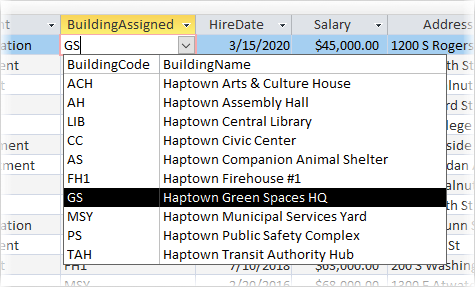
- We want to have the BuildingAssigned field be a drop-down selector that lists the buildings in our database.
- Temporarily change the data type to Lookup Wizard
- Select the BuildingID, BuildingCode, and BuildingName fields
- Sort ascending by BuildingName only, and Hide the primary key
- In Lookup properties, change the second column to 3″ and the total column width to 4″
- Also enable Column Heads and choose Yes for Limit To List
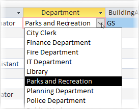
- Let’s do the same thing for the Department field from tblDepartment.
- Select the Department field only, sorting by that field
- Set the column and list width to 2″
- No Column Heads, but Yes for Limit To List
Save and close the tblEmployee table.
tblAsset, tblBuilding tables
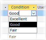
- For both tbleAsset and tblBuilding, let’s make the Condition field a drop-down list of options listing Excellent, Good, and Fair.
- No Column Heads, but Yes for Limit To List
Save and close each table when complete.
tblTicketData table
- Create a new field named officer that is a Lookup Wizard type.
- Lookup data in tblEmployee and select the EmployeeID, LastName, and JobTitle fields.
- Sort by LastName and hide the ID field
- Set the second column to 2″ and the overall width to 3″
- Set Column Heads and Limit To List both to Yes
Does it make sense that we can select all employees for this field? We will address this in Chapter 4.
Save and close the tblTicketData table.
tblAssignedSoftware Composite Key
We want this to be what we call a Junction Table. This will just store pairs of what we call Foreign Keys from the Software and Employee tables. What we want is for an employee to be assigned a software package only once – an employee can never be assigned the same software. Because of this, we will set both fields herein as the primary key, or what we call a Composite Key.
Select both fields at the same time and click the Primary Key button in the ribbon.
Save and close the tblAssignedSoftware table.
Relationship Details
First, let’s create relationships in a different way in our Relationships tool. Open this up and click All Relationships in the ribbon. If necessary, click and drag tblAssignedSoftware to the diagram canvas area. Then, click and drag SoftwareID from tblSoftware to the same field name in tblAssignedSoftware. Do the same for EmployeeID from tblEmployee.
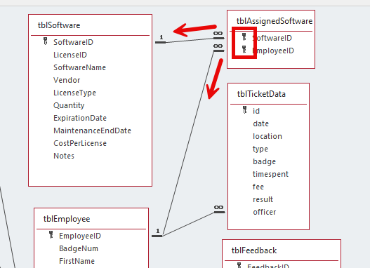
When two or more tables are used in a query, those tables need to be related to each other in the database. For each relationship we created above, Enforce Referential Integrity and Cascade Update Related Fields.
Save your relationships diagram when you are finished editing it.
Make sure all objects are closed. Close the database. Double-check the Last Modified date for your database file.
More Practice
Work you should do before our next class
Go to your IU OneDrive and open your username-Haptown database.
tblMarketVendor table
- Create a lookup for the PrimaryDepartment field to tblDepartment
- Select the Department field only, sorting by that field
- Set the column and list width to 2″
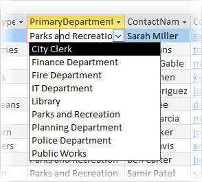
Save and close the tblMarketVendor table.
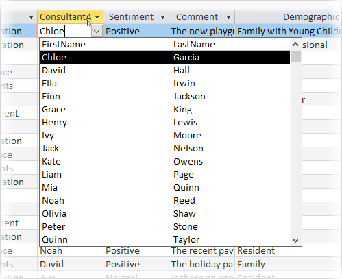
tblFeedback table
- Create a lookup for ConsultantAssigned from tblConsultant
- Select ConsultantID, LastName, and FirstName (in that order)
- Order by LastName then FirstName
- Do not show the ID field
- Set the column and list widths to 2″
- Display Column Heads and enable Limit To List
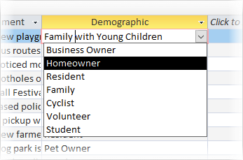
- Create a manual value list drop-down for Demographic. Do NOT use Limit To List but select Yes for Allow Value List Edits. This is so people can add other Demographic entries if needed. Use the following options in your list.
- Business Owner
- Cyclist
- Family
- Homeowner
- Resident
- Student
- Volunteer
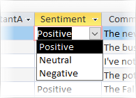
- Make the Sentiment field a drop-down list of options listing Positive, Neutral, and Negative. No Column Heads, but Yes for Limit To List
Save and close the tblFeedback table.
Relationship Details
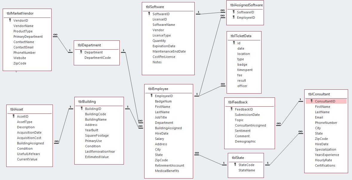
When two or more tables are used in a query, those tables need to be related to each other in the database. Create relationships between the tables in this database according to the image below. For each relationship, Enforce Referential Integrity and Cascade Update Related Fields.
Save your Relationships diagram when you are finished editing it.
Make sure all objects are closed. Close the database. Double-check the Last Modified date for your database file.
Post-Chapter 2 ERD
Your Entity Relationship Diagram (ERD, also known as the “Relationships” tool in Access) should look something like this after the Chapter 2 contents. We may do more work on the other desired relationships later.