Interpolation and Polynomial Approximation

Donovan D Chang

31 Interpolation and Polynomial Approximation

In this section, we discuss methods to approximate a function with polynomials, and estimating the value of the function where its value is unknown. Estimating the value between the given, i.e. known, data points is called interpolation, and outside, the value of unknown points, is called extrapolation. Indeed, interpolation is less-prone to error, and likely error will be smaller near the known data points. As such, we need to exercise caution in extrapolation, as the behavior of fitted curve or approximating polynomial may be far off from the real function.

Also, the function of interest may or may not be known. When the function is known, our goal would be obtaining reasonably accurate estimates with much less burden of computation. One famous example, though not applicable to every function, is the Taylor expansion. Note the motivation of developing Taylor expansion was to express differentiable non-polynomial functions as a polynomial.

A familiar example of approximating an unknown function would be interpolation and extrapolation with census data. Due to its expensive resource consumption, census is not conducted annually but at several years of interval. In fact, while usually is the case the census bureau interpolates population of intercensal period with an exponential function, for illustration purpose, here we shall estimate with a polynomial.

We begin this section by introducing the method, the Lagrange interpolating polynomial.

Interpolation and the Lagrange Polynomial

The $n$ -th Lagrange interpolating polynomial is the formula to construct a unique polynomial connecting $n+1$ distinct points.

Theorem. ( $n$ -th Lagrange Interpolating Polynomial [7])
Given $(x_i,y_i)\in f$ for $i=0,1,2,\cdots,n$ , the $n$ -th Lagrange interpolating polynomial $P_n(x)$ is a unique polynomial of at most degree $n$ satisfying $P_n(x_i)=y_i=f(x_i)$ given by

$\begin{align*} P_n(x) &= \sum^n_{i=0}y_iL_i(x)\\ &= y_0L_0(x)+y_1L_1(x)+\cdots +y_nL_n(x) \end{align*}$

where

$\begin{align*} L_i(x) &= \prod^n_{k=0,k\neq i}\frac{x-x_k}{x_i-x_k}\\ &= \frac{(x-x_0)(x-x_1)\cdots (x-x_{i-1})(x-x_{i+1})\cdots (x-x_n)}{(x_i-x_0)(x_i-x_1)\cdots (x_i-x_{i-1})(x_i-x_{i+1})\cdots (x-x_n)} \end{align*}$

Let us illustrate with an example.

Example. Estimating U.S. Population in 2020

Following are the historical U.S. population data from the U.S. Census Bureau [1].

$\begin{array}{c|c} \text{Year} & \text{Population in Millions} \\ \hline 1990 & 249 \\ 2000 & 281 \\ 2010 & 309 \end{array}$

Using the Lagrange interpolating method, estimate the U.S. population in 2005 and 2020.

We have 3 data points. Therefore, the Lagrange polynomial, where $x$ is year, will be of a second order as follows:

$\begin{align*} P_2(x) &= 249\frac{(x-2000)(x-2010)}{(1990-2000)(1990-2010)} + 281\frac{(x-1990)(x-2010)}{(2000-1990)(2000-2010)}\\ &\quad + 309\frac{(x-1990)(x-2000)}{(2010-1990)(2010-2000)}\\ &= \frac{249}{200}(x-2000)(x-2010) \quad \quad \;\;\; - \frac{281}{100}(x-1990)(x-2010)\\ &\quad + \frac{309}{200}(x-1990)(x-2000) \end{align*}$

Therefore,

$\begin{align*} P_2(2005) &= 295.5 \approx 296\\ P_2(2020) &= 333 \end{align*}$

Therefore, the estimated U.S. population in 2005 and in 2020 are approximately 296 and 333 millions, respectively.

Now, let us have a look at another example of a known function.

Example. Construct a Lagrange interpolating polynomial $P(x)$ of $f(x)=\frac{1}{x}$ with the nodes $x=2,4,8$ , and examine the accuracy of $P(1)$ and $P(3)$ .

Let us construct the Lagrange polynomial first. As we have 3 data points, $\left(2,\frac{1}{2}\right)$ , $\left(4,\frac{1}{4}\right)$ , and $\left(8,\frac{1}{8}\right)$ , the Lagrange polynomial will be in the second order as follows:

$\begin{align*} P_2(x) &= \frac{1}{2}\frac{(x-4)(x-8)}{(2-4)(2-8)} + \frac{1}{4}\frac{(x-2)(x-8)}{(4-2)(4-8)} + \frac{1}{8}\frac{(x-2)(x-4)}{(8-2)(8-4)}\\ &= \frac{1}{24}(x-4)(x-8) - \frac{1}{32}(x-2)(x-8) + \frac{1}{192}(x-2)(x-4) \end{align*}$

Therefore,

$\begin{align*} P_2(1) &= \frac{129}{192} = 0.671875\\ P_2(3) &= \frac{69}{192} = 0.359375 \end{align*}$

Therefore, errors are

$\begin{align*} \varepsilon_{x=1} &= \widehat{f(1)}-f(1)\\ &= P_2(1)-f(1)\\ &= -0.328125\\ \varepsilon_{x=3} &= \widehat{f(3)}-f(3)\\ &= P_2(3)-f(3)\\ &= 0.0260416666\cdots\\ &= 0.026041\dot{6} \end{align*}$

Unlike the previous example of estimating U.S. population, we observe errors in our estimates. Note that $|\varepsilon_{x=1}|>|\varepsilon_{x=3}|$ . In fact, the magnitude of error is much larger at $x=1$ than at $x=3$ . This is within our expectation that the farther away the interpolating or extrapolating points are located from the data points we know, the more error there likely is.

Error Analysis of Lagrange Polynomial

The remainder term for Lagrange polynomial is a derivation of the truncation error of Taylor expansion. First, let us restate the Taylor polynomial as follows:

$\begin{align*} R_n(x) &= f(x)-P_n(x)\\ &= \frac{f^{(n+1)}(\xi)}{(n+1)!}(x-x_0)^{(n+1)} \end{align*}$

where $P_n(x)$ denotes the $n$ -th order Taylor polynomial.

The Lagrange polynomial uses information from $n+1$ different points rather than a single point $x_0$ in Taylor expansion. Therefore, we obtain the remainder term of Lagrange polynomial by replacing $(x-x_0)^{(n+1)}$ with $\prod^n_{i=0}(x-x_i)$ as follows:

The truncation error $R(x)$ of $n$ -th order Lagrange polynomial is

$\begin{align*} R(x) &= f(x)-P_n(x)\\ &= \frac{f^{(n+1)}(\xi)}{(n+1)!}\prod^n_{i=0}(x-x_i) \end{align*}$

where $P_n(x)$ denotes the $n$ -th order Lagrange polynomial.

Let us illustrate with an example.

Example. Determine the maximum possible error, i.e. error bound, of the previous example.

The truncation error $R(x)$ of the 2nd order Lagrange polynomial is

$\begin{align*} R(x) &= f(x)-P_2(x)\\ &= \frac{f'''(\xi)}{3!}(x-x_0)(x-x_1)(x-x_2)\\ &= -\frac{6(\xi^{-4})}{3!}(x-2)(x-4)(x-8)\\ &= -\xi^{-4}(x-2)(x-4)(x-8) \end{align*}$

Then, for $\xi\in [2,8]$ ,

$\left\vert \xi^{-4}\right\vert = \frac{1}{\xi^{4}}\leq \frac{1}{2^4} = \frac{1}{16}$

Therefore,

$\begin{align*} \left\vert R(x) \right\vert &= \left\vert f(x)-P_2(x) \right\vert\\ &= \left\vert -\xi^{-4}(x-2)(x-4)(x-8) \right\vert\\ &\leq \left\vert \frac{1}{16}(x-2)(x-4)(x-8) \right\vert \end{align*}$

Let $g(x) =(x-2)(x-4)(x-8)$ .
Then, $g'(x) = 3x^2-28x+56$ .
Then, $g'$ has a local minimum and maximum at

$\begin{align*} x &= \frac{14\pm \sqrt{14^2-3\cdot 56}}{3}\\ &= \frac{14\pm 2\sqrt{7}}{3} \end{align*}$

Therefore, the max of $\left\vert g(x)\right\vert$ on $[2,8]$ is at $x=\frac{14+ 2\sqrt{7}}{3}$ .
Therefore, for $x\in [2,8]$ ,

$\begin{align*} \left\vert R(x) \right\vert &\leq \left\vert \frac{1}{16}\left(x-2\right)\left(x-4\right)\left(x-8\right) \right\vert\\ &\leq \left\vert \frac{1}{16}\left(\frac{14+ 2\sqrt{7}}{3}-2\right)\left(\frac{14+ 2\sqrt{7}}{3}-4\right)\left(\frac{14+ 2\sqrt{7}}{3}-8\right) \right\vert\\ &\approx 1.056305895 \end{align*}$

Therefore, the maximum error of $P_2(x)$ for $\frac{1}{x}$ on $[2,8]$ is approximately 1.06.

Divided Difference

We have explored a little bit of interpolating polynomials. However, the downside of constructing a Lagrange polynomial is it is computationally expensive. That is, constructing a second order polynomial with only 3 data points was already bulky, and as reflected in the formula of Lagrange interpolating polynomial, the computation required increases exponentially as we have more data points. Therefore, another method requiring less calculation, or more efficient mechanism, was developed by Newton, and is called Newton’s divided-difference formula or Newton’s interpolating polynomial.

Theorem. (Newton’s Interpolating Polynomial)
The $n$ -th Lagrange interpolating polynomial $P_n(x)$ penetrating $(x_i,y_i)\in f$ of a continuous function $f$ for $i=0,1,2,\cdots,n$ is unique, but also can be expressed in an alternative form, Newton’s interpolating polynomial as follows:

$\begin{align*} P_n(x) &= a_0+\sum^n_{k=1}a_k\prod^{k-1}_{j=0}(x-x_j)\\ &= a_0+a_1(x-x_0)+a_2(x-x_0)(x-x_1)+\cdots\\ &\quad +a_n(x-x_0)(x-x_1)\cdots(x-x_{n-1}) \end{align*}$

where $a_0=f(x_0)$ and $a_n$ denotes the $n$ -th divided difference of $f$ defined as
$a_n = f[x_0,x_1,x_2,\cdots,x_n] = \frac{f[x_1,x_2,\cdots,x_n]-f[x_0,x_1,\cdots,x_{n-1}]}{x_n-x_0}$

Proof.
First, write a $n$ -th polynomial $P_n(x)$ as follows:

$\begin{align*} P_n(x) &= a_0+a_1(x-x_0)+a_2(x-x_0)(x-x_1)+\cdots\\ &\quad +a_n(x-x_0)(x-x_1)\cdots(x-x_{n-1}) \end{align*}$

Then, determine the coefficient $a_i$ ‘s where $i=0,1,2,\cdots,n$ .

$a_0 = p_n(x_0)=f(x_0)$

$a_1=\frac{f(x_1)-f(x_0)}{x_1-x_0}$ , since $P_n(x_1)=f(x_0)+a_1(x_1-x_0)=f(x_1)$

$a_2 = \frac{\frac{f(x_2)-f(x_0)}{x_2-x_0}-a_1}{x_2-x_1}$ , since $P_n(x_2)=f(x_0)+a_1(x_2-x_0)$
$\quad\quad\quad\quad\quad\quad\quad\quad\quad\quad\quad\quad\quad\quad\quad +a_2(x_2-x_0)(x_2-x_1)=f(x_2)$

$\vdots$

Next, introduce the divided difference notation.
The 0th divided difference of $f$ is

$f[x_i] = f(x_i)$

The 1st divided difference of $f$ is

$f[x_i,x_{i+1}] = \frac{f[x_{i+1}]-f[x_i]}{x_{i+1}-x_i}$

The 2nd divided difference of $f$ is

$f[x_i,x_{i+1},x_{i+2}] = \frac{f[x_{i+1},x_{i+2}]-f[x_i,x_{i+1}}{x_{i+2}-x_i}$

$\vdots$

The $k$ -th divided difference of $f$ is

$f[x_i,x_{i+1},\cdots,x_{i+k}] = \frac{f[x_{i+1},x_{i+2},\cdots,x_{i+k}]-f[x_i,x_{i+1},\cdots,x_{i+k-1}]}{x_{i+k}-x_i}$

By letting $i=0$ and $k=n$ , we have the $n$ -th divided difference of $f$ as follows:

$f[x_0,x_{1},\cdots,x_{n}] = \frac{f[x_{1},x_{2},\cdots,x_{n}]-f[x_0,x_{1},\cdots,x_{n-1}]}{x_{n}-x_0}$

Then, we have

$\begin{align*} a_0 &= f[x_0]\\ a_1 &= f[x_0,x_1]\\ &\vdots\\ a_n &= f[x_0,x_{1},\cdots,x_{n}] \end{align*}$

Finally, express the coefficients $a_i$ ‘s in divided difference notation

$\begin{align*} P_n(x) &= f[x_0]+\sum^n_{k=1}f[x_0,x_{1},\cdots,x_{k}]\prod^{k-1}_{j=0}(x-x_j)\\ &= f[x_0]+f[x_0,x_1](x-x_0)+f[x_0,x_1,x_2](x-x_0)(x-x_1)+\cdots\\ &\quad +f[x_0,x_{1},\cdots,x_n](x-x_0)(x-x_1)\cdots(x-x_{n-1}) \end{align*}$

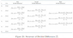
The following table shows the generation of divided differences. Note that the order of inputs, i.e. $x_i$ ‘s are irrelevant.

Let us conclude this section with an illustrative example.

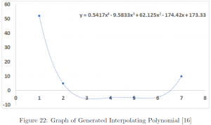
Example. Find the Newton’s interpolating polynomial of the following dataset.

$\begin{array}{c|ccccc} x & 1 & 2 & 4 & 5 & 7 \\ \hline y & 52 & 5 & -5 & -5 & 10 \end{array}$

First, we construct a divided difference table.

$\begin{array}{cc|cccc} x &y &d_1 &d_2 &d_3 &d_4\\ \hline 1 &52 &-47.0000 &14.0000 &-3.0833 &0.541666667\\ 2 &5 &-5.0000 &1.6667 &0.1667\\ 4 &-5 &0.0000 &2.5000\\ 5 &-5 &7.5000\\ 7 &10\\ \end{array}$

Detailed calculations in the following steps are overly complex to be carried out by hand, and thus omitted. Also, note that the aim of this summary is to understand important concepts and theorems, and know how to apply those. The author recommends the use of a computer package such as Python, Wolfram Mathematica, SAS, R, and Stata. Following is the result with a graph generated using Microsoft Excel 2020.

Cubic Spline Interpolation

Computational challenge of constructing a high-order Lagrange interpolating polynomial has been substantially reduced with the introduction of Newton’s method using divided difference, a method of sequentially adding information than to use all data points all at once.

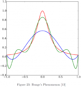
However, another problem occurs called Runge’s phenomenon, the problem of oscillation at the edges of fitted polynomial, especially when fitting a polynomial with equally spaced nodes (Figure 23). The red curve in the figure denotes the Runge’s function, the blue curve is a polynomial fitted with 5 data points, and the green curve fitted with 9 data points. It is contrary to the general trend of increasing accuracy with more data points, but the oscillations at the edges result in substantial increase in errors. To resolve this issue, in this section we introduce piecewise interpolation.

The simplest form would be a piecewise linear function, simply “connecting the dots.” However, we omit this case, a series of straight lines, as this is a rudimentary form that is only continuous, but highly unlikely to be differentiable at the nodes. An advanced form is a piecewise-quadratic function. Constructing a series of second order polynomial connecting the points, so that the tangent evaluated at the nodes would agree in adjacent functions. Let us have a look at the simplest example with only 3 nodes.

Let $(x_i,y_i)$ be the nodes for $i=0,1,2$ . Then, to fit a piecewise-quadratic function, we need to construct 2 polynomials, $Q_0$ and $Q_1$ , satisfying the following conditions:

$\begin{cases} Q_0(x_0) = y_0\\ Q_0(x_1) = y_1 = Q_1(x_1)\\ Q_1(x_2) = y_2\\ Q'_0(x_1) =Q'_1(x_1) \end{cases}$

Note that there may be many polynomials satisfying the conditions above, i.e. the polynomial is not uniquely determined. Therefore, in general, an additional condition is given such as the derivative at one of the endpoints. However, the difficulty is we usually do not have enough information on the derivatives on the endpoints.

Another way, in fact the most commonly used piecewise polynomial, is the piecewise-cubic or cubic spline method, fitting cubic functions connecting specified nodes with a series of cubic function. The main advantage of this method is it may provide a smoother function by requiring the same concavity at each connecting node, yet at the cost of increased computations. Following is the general form of a cubic spline:

Let $(x_i,y_i)$ be nodes for the cubic spline for $i=0,1,2,\cdots,n$ and denote each cubic polynomial as $S_j(x)$ for $j=0,1,2,\cdots,n-1$ , satisfying

$\begin{cases} S_j(x_j) &= y_j\\ S_{j+1}(x_{j+1}) &= y_{j+1}\\ S_{j}(x_{j+1}) &= S_{j+1}(x_{j+1})\\ S'_{j}(x_{j+1}) &= S'_{j+1}(x_{j+1})\\ S''_{j}(x_{j+1}) &= S''_{j+1}(x_{j+1})\\ \end{cases}$

and one of

$\begin{cases} S''(x_0)=S''(x_n)=0 &\text{natural or free boundary}\\ S'(x_0)=f'(x_0) \text{ and } S'(x_n)=f'(x_n) &\text{clamped boundary} \end{cases}$

Let us conclude this section with an illustrative example.

Example. Construct a clamped cubic spline of $f$ interpolating $(1,2)$ , $(2,3)$ , and $(3,5)$ , where $f'(1)=2$ and $f'(3)=1$ .

Let $S_j(x) = a_j+b_jx+c_jx^2+d_jx^3$ for $j=0,1$ .
Then, we have

$\begin{cases} S'_j(x) &= b_j+2c_jx +3d_jx^2\\ S''_j(x) &= 2c_j +6d_jx \end{cases}$

We need to find polynomials $S_0(x)$ and $S_1(x)$ satisfying

$\begin{cases} S_0(x_0) &= y_0\\ S_0(x_{1}) &= y_{1}\\ S_1(x_1) &= y_1\\ S_{1}(x_{2}) &= y_{2}\\ S'_{0}(x_{0}) &= y'_0\\ S'_{1}(x_{2}) &= y'_2\\ S'_{0}(x_{1}) &= S'_{1}(x_{1})\\ S''_{0}(x_{1}) &= S''_{1}(x_{1})\\ \end{cases}$

Solving the linear system above, the yielded cubic polynomials are

$\begin{cases} S_0(x)= 2+2(x-1)-2.5(x-1)^2+1.5(x-1)^3 &1\leq x\leq 2\\ S_1(x)= 3+1.5(x-2)+2(x-2)^2-1.5(x-2)^3 &2\leq x\leq 3 \end{cases}$

Note that actual calculations were omitted. As the number of nodes increases, the required amount of computations involved rapidly increases accordingly. As such, sound judgement is required for the “tradeoff” between fitting a cubic spline vs a $n$ -th order interpolating polynomial.

31 Interpolation and Polynomial Approximation

Interpolation and the Lagrange Polynomial

Error Analysis of Lagrange Polynomial

Divided Difference

Cubic Spline Interpolation

License

Share This Book