Limits and Continuity

Donovan D Chang

1 Limits and Continuity

To discuss integration and differentiation, we need to introduce and understand the notions of limits and continuity. Let us begin with an intuitive definition of a limit from the Stewart’s Calculus Textbook.

Definition (Intuitive Definition of Limit)
Suppose $f(x)$ is defined on an interval $(a,b)\subseteq \mathbb{R}$ , and let $z\in (a,b)$ . When $x$ is near $z$ , and the value of $x$ is near $L$ , then we write

$\lim_{x\to z} f(x)=L$

and say “the limit of $f(x)$ , as $x$ approaches $z$ , equals $L$ .

As implied from the way how limit is read, the limit of $f(x)$ at $z$ equals $L$ in fact means

“the value of $f$ approaches $L$ , as $x$ approaches $z$ .”

Note on Nearness

It is critical to note $\lim_{x\to z}f(x)=L$ is different from $f(z)=L$ . In fact, for the limit of $f$ to be defined, $f$ need only be defined near $z$ , but not at $z$ itself. Then, we might as well wonder what we mean by one value is near some other value, i.e. to what extent we might call one is near the other and from which point not near. This ambiguity around nearness will later be removed with the formal $\delta$ – $\epsilon$ definition of a limit, as well as with the concept of neighborhood.

Let us look at an example.

Example. Evaluate $\lim_{x\to 0} \frac{x^3}{x}$

Let $f(x)=\frac{x^3}{x}$ .
We note that $f(x)$ is defined on $\mathbb{R}\setminus \lbrace 0 \rbrace$ , and thus $f(0)$ is not defined. Still, we can evaluate the limit of $f(x)$ at $x=0$ , since $f$ is defined near 0. Let us have a look at the graph of $f(x)$ :

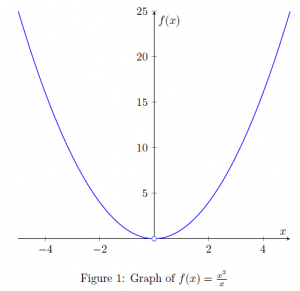
We observe $\frac{x^3}{x}$ approaches 0, as $x$ approaches 0 (Figure ??). Therefore,

$\begin{align*} \lim_{x\to 0} \frac{x^3}{x} &= \lim_{x\to 0} x^2\\ &= 0 \end{align*}$

The cancellation of $x$ is valid, since $x\neq 0$ by the definition of limit.

Our discussion of limit so far has been on the intuitive definition that the value of the function $f(x)$ approaches a certain value, $L$ , as $x$ approaches to the point where the limit is being evaluated, $z\in (a,b)$ in our previous example. In fact, except where the limit is evaluated on the edge of a given interval, the value can be approached from both sides. That is, there are left-hand and right-hand limits. Let us examine the left-hand and right-hand limits at various points of a discontinuous function $g(x)$ defined by

$g(x)= \begin{cases} x^2 & (x<2) \\ x & (2\leq x <4) \\ -x+6 & (x\geq 4) \end{cases}$

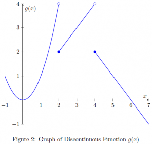
We observe $g$ , defined on $\mathbb{R}$ , is discontinuous at 2 points, at $x=2$ and $x=4$ . In these cases, the limit is not defined, as the values near the point of interest, or the values of $g$ approached from the left and from the right, are not the same. When we say approaching $g$ from the left and from the right, they correspond to inputting values of $x$ , close to the point of interest, while less than and greater than, respectively.

While $g(2)=2$ , when $g$ is approached from the left around 2, the value approaches 4. In this case, we say, “the left-hand limit of $g(x)$ at 2 is 4,” and write

$\lim_{x\to 2-0} g(x)=4 \text{ or } \lim_{x\to 2^-} g(x)=4 \text{,}$

omitting 0 after the negative sign ( $-$ ). Note that the zero after the negative sign denotes an arbitrarily small, but positive, value but not equal to 0.

Likewise, we can evaluate the right-hand limit of $g$ at 2 as the value of $g$ near, but slightly greater than, 2, and write

$\lim_{x\to 2+0} g(x) = \lim_{x\to 2^+} g(x) = 2$

Note that

$\begin{align*} & \lim_{x\to 2-0} g(x) = 4\\ \neq & \lim_{x\to 2+0} g(x) = 2 \end{align*}$

As above, in the cases where the values of the left-hand limit and the right-hand limit are not equal, we say the limit is not defined and divergent.

Let us discuss another divergent case, where the limit diverges to positive or negative infinity. One such function is $h(x)=\frac{1}{x}$ . We know division by zero is not defined, and thus the domain of $h$ is non-zero real numbers, i.e. $\mathbb{R}\setminus \lbrace 0 \rbrace$ . However, $h$ is defined on any number close to or near 0, no matter how small its absolute value is. Let us construct a table and observe a pattern:

(1) $\begin{equation*} \begin{array}{c|ccccccc|c} x & \cdots & -1 & -0.1 & -0.01 & -0.001 & -0.0001 & \cdots & 0 \\ \hline h(x) & 0^- & -1 & -10 & -100 & -1000 & -10000 & -\infty & \emptyset \end{array} \end{equation*}$

(2) $\begin{equation*} \begin{array}{c|c|ccccccc} x & 0 & \cdots & +0.0001 & +0.001 & +0.01 & +0.1 & +1 & \cdots \\ \hline h(x) & \emptyset & \infty & +10000 & +1000 & +100 & +10 & +1 & 0^+ \end{array} \end{equation*}$

In the equation (2), we observe $h$ decreases and approaches 0 in the positive domain $\left( \mathbb{R}^+ \right)$ , as the value of $x$ increases in $\mathbb{R}^+$ towards infinity. When $x$ decreases in $\mathbb{R}^+$ and approaches 0, we see a rapid increase in $h(x)$ without a bound, i.e. $h(x)\rightarrow \infty$ .

The pattern found in the equation (1) is similar. A decrease in the magnitude of $x$ in the negative domain $\left( \mathbb{R}^- \right)$ results in the rapid increase in the magnitude of $h(x)$ , which also is in $\mathbb{R}^-$ . The absolute value of $h(x)$ becomes smaller and approaches 0 in $\mathbb{R}^-$ with a decrease of $x$ in $\mathbb{R}^-$ .

The similar pattern observed in the equations (1) and (2) is owing to the fact $h(x)=\frac{1}{x}$ is an odd function, i.e. $h(-x)=-h(x)$ . We can see the symmetry about the origin in the plot (Figure 3).

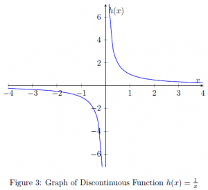
Following is the evaluation of limits at the singularities of $h(x)$ , where $h(x)=\frac{1}{x}$ is not defined but the limit is defined:

$\begin{cases} \lim_{x\to \infty} \frac{1}{x} &= 0\\ \lim_{x\to -\infty} \frac{1}{x} &= 0\\ \lim_{x\to 0^-} \frac{1}{x} &= -\infty\\ \lim_{x\to 0^+} \frac{1}{x} &= +\infty\\ \lim_{x\to 0} \frac{1}{x} &= \emptyset \end{cases}$

Note the limit of $\frac{1}{x}$ at $x=0$ is not defined.

Our discussion of left-hand and right-hand limits can be succinctly summarized as follows:

$\lim_{x\to a} f(x)=L$

iff $\lim_{x\to a^+} f(x)=L$ and $\lim_{x\to a^+} f(x)=L$

So far we have covered three cases as follows:

The left-hand and right-hand limits are the same, and thus the limit at the point is defined; and the value of the function where the limit is evaluated is the same as the limit;
Same as above, but the value of the function where the limit is evaluated is not defined or not equal to the limit; and
The left-hand and right-hand limits are not the same.

Per case 1., the left-hand and right-hand limits are the same, and thus the limit at the point is defined; and the value of the function where the limit is evaluated is the same as the limit, we call the function is continuous at the evaluated point. Before moving onto the formal definition of a continuous function, precise definition of a limit is provided here.

Definition. ( $\delta$ – $\epsilon$ Definition of Limit)

Let $f$ be a function defined on some open interval that contains the number $a$ , except possibly at $a$ itself. Then we say the limit of $f(x)$ , as $x$ approaches $a$ , is $L$ , and we write

$\lim_{x\to a} f(x)=L$

if for every number $\epsilon>0$ there is a number $\delta>0$ such that

if $0<|x-a|<\delta$ , then $|f(x)-L|<\epsilon$ .

Above definition is commonly referred to as $\delta$ – $\epsilon$ definition of a limit. With a bit of algebraic manipulation, the conditional inequalities can be equivalently expressed as follows:

$\left(\forall \epsilon\in \mathbb{R}^+ \right) \left(\exists \delta\in \mathbb{R}^+ \right) \left( a-\delta <x<a+\delta \right) \Rightarrow \left(L-\epsilon <f(x)<L+\epsilon\right)$

which translates to, “for any value of $f(x)$ arbitrarily close to $L$ , there exists $x$ around $a$ , where the interval around $a$ with a radius $\delta$ is within the domain.”

Therefore, it follows that the substitution of antecedent with $\left( a-\delta <x<0 \right)$ and $\left( 0 <x<a+\delta \right)$ corresponds to the $\delta$ – $\epsilon$ definition of the left-hand and the right-hand limits, respectively, since by forcing one of the interval endpoints around $x$ to 0, approaching towards $x$ becomes one-sided.

We recapitulate as follows

Definition. ( $\delta$ – $\epsilon$ Definition of Left-Hand Limit)

We write the left-hand limit of $f(x)$ at $a$ is $L$ as

$\lim_{x\to a^-} f(x)=L$

if for every number $\epsilon>0$ there is a number $\delta>0$ such that $\left( a-\delta <x<0 \right) \Rightarrow \left(|f(x)-L|<\epsilon\right)$ .

Definition. ( $\delta$ – $\epsilon$ Definition of Right-Hand Limit)

We write the right-hand limit of $f(x)$ at $a$ is $L$ as

$\lim_{x\to a^+} f(x)=L$

if for every number $\epsilon>0$ there is a number $\delta>0$ such that $\left( 0 <x<a+\delta \right) \Rightarrow \left(|f(x)-L|<\epsilon\right)$ .

Let us illustrate the definition with an example.

Prove that $\lim_{x\to 2} x^2=4$ .

1. Guessing a value for $\delta$ .

Let $\epsilon>0$ be given. We have to find a number $\delta>0$ such that

$\begin{array}{cll} & \left( 0<|x-2|<\delta \right) &\Rightarrow |x^2-4|<\epsilon \\ \text{iff} & \left( 0<|x-2|<\delta \right) &\Rightarrow |(x-2)(x+2)|<\epsilon \end{array}$

Suppose $|x+2|<C$ , where $C>0$ . Then,

$|x+2||x-2|<C|x-2|$

Then, we can make $C|x-2|<\epsilon$ by letting $|x-2|<\frac{\epsilon}{C}$ , so we could choose $\delta=\frac{\epsilon}{C}$ .

Let $|x-2|<1$ . Then, $1<x<3$ , and thus $3<x+2<5$ . Therefore, we have $|x+2|<5$ , and so $C=5$ is a suitable choice for the constant.

Then,

$|x-2|<1 \text{ and } |x-2|<\frac{\epsilon}{C}=\frac{\epsilon}{5}$

To ensure both inequalities above are satisfied, let $\delta=\text{min}\{1,\frac{\epsilon}{5}\}$ .

2. Showing that this $\delta$ works.

Let $\delta=\text{min}\{1,\frac{\epsilon}{5}\}$ for $\epsilon>0$ .

If $0<|x-2|<\delta$ , then

$\begin{array}{cl} & |x-2|<1\\ \Rightarrow & 1<x<3\\ \Rightarrow & |x+2|<5 \text{ (as in part 1)} \end{array}$

Also, $|x-2|<\frac{\epsilon}{5}$ . Therefore,

$|x^2-4|=|x+2||x-2|<5\cdot\frac{\epsilon}{5}=\epsilon$

We have just shown, for every number $\epsilon>0$ , there is a number $\text{min}\{1,\frac{\epsilon}{5}\}>0$ such that $\left( |x-2|<\text{min}\{1,\frac{\epsilon}{5}\} \right) \Rightarrow \left(|x^2-4|<\epsilon\right)$ . Therefore, by definition of $\delta$ – $\epsilon$ limit, we conclude $\lim_{x\to 2} x^2=4$ .

Now we turn to continuity of a function. A continuous function is succinctly defined as

Definition. (Continuity)
A function $f$ is continuous at a number $a$ if

$\lim_{x\to a} f(x)=f(a)$

In fact, above definition implies the following:

$f(a)$ is defined (that is, $a \in \mathrm{Dom}(f)$ );
$\lim_{x\to a} f(x)=f(a)$ exists; and
$\lim_{x\to a} f(x)=f(a)$

Likewise, it follows that

Definition. (Left- and Right-Continuity)
A function $f$ is continuous from the right at a number $a$ if

$\lim_{x\to a^+} f(x)=f(a)$

and $f$ is continuous from the left at a number $a$ if

$\lim_{x\to a^-} f(x)=f(a)$

So far we have only discussed the continuity of a function at a given point. In fact, the notion of continuity can be expanded to an interval, and we call this a continuous function. Following is a formal definition from Stewart [10]

Definition. (Continuous Function)
A function $f$ is continuous on an interval if it is continuous for all the numbers in the interval.

In this section, we began our discussion with an intuitive definition of a limit, and familiarized ourselves with limit through a few examples of left-hand and right-hand limits, and divergent cases. Then, we provided a refined and formal definition of a limit using $\delta$ and $\epsilon$ , and defined continuity of a function.

Now we are ready to discuss derivatives, the topic to be dealt in the following chapter, concerning the rate of change, where the prerequisite is a given function to be continuous. Let us delve in.

1 Limits and Continuity

License

Share This Book