Multivariate Calculus

Donovan D Chang

5 Multivariate Calculus

So far we have been discussing the calculus of a univariate function, where there is a single independent variable for a dependent variable. In this section, we expand our purview to the functions with multiple independent variables – two, three, or more.

First, let us consider a bivariate function $f$ of two independent variables defined by

$\left\lbrace f(x,y)\, \vert \, (x,y)\in D \right\rbrace$

where $D \subset \mathbb{R}\times\mathbb{R}$ . Often we write in the form of $z=f(x,y)$ , and thus $z$ is a dependent variable with independent variables $x$ and $y$ . By adding $z$ -axis to the $x$ – $y$ coordinate plane, we can envisage the function in a 3-dimensional plane.

The same notion applies to a function with $n$ independent variables, though visual representation becomes a challenge. A function $f$ with $n$ independent variables would take the form of

$y=f(x_1,x_2,\cdots,x_n)$

where $(x_1,x_2,\cdots,x_n)\in \mathbb{R}^n$ .

Partial Differentiation

Imagine a mountain placed on a $x$ – $y$ – $z$ coordinate plane. Suppose we are interested in examining the relationship between the height $z$ and the rest of the coordinates $x$ and $y$ . That is, we consider a function $z=f(x,y)$ , where $z$ is a dependent variable and $x$ and $y$ are independent variables. What if we are interested in the rate of change in $z$ to the change in $x$ or $y$ ? This is the moment we need to introduce the concept of partial differentiation.

A partial derivative of a multivariate function is defined as a derivative of function with respect to one of the independent variables, while holding the rest of independent variables constant. Suppose we are interested in the relationship between $x$ and $z$ holding $y$ constant. Then, the partial derivative of $z$ with respect to $x$ is

$f_{x} =\lim_{h \to 0}\frac{f(x+h,y)-f(x,y)}{h}$

Likewise,

$f_{y} =\lim_{h \to 0}\frac{f(x,y+h)-f(x,y)}{h}$

Different notations for partial derivatives are as follows:

$f_{x}(x,y) =f_{x} =\frac{\partial f}{\partial x} =\frac{\partial}{\partial x}f(x,y)=\frac{\partial z}{\partial x}=z_{x}=D_{1}f=D_{x}f$

Now, let us illustrate with a few examples.

Example. Find $f_x(x,y)$ and $f_{x}(1,2)$ of $f(x,y)=x^3+2x^2y+y^2$ .

$\begin{align*} f_x(x,y) &= 3x^2+4xy\\ f_x(1,2) &= 3(1)^2+4(1)(2)\\ &= 11 \end{align*}$

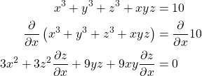
Example. Find $\frac{\partial z}{\partial x}$ of $x^3+y^3+z^3+9xyz=10$ implicitly, where $z$ is a function of $x$ and $y$ .

$\begin{align*} x^3+y^3+z^3+xyz &= 10\\ \frac{\partial }{\partial x}\left( x^3+y^3+z^3+xyz\right) &=\frac{\partial }{\partial x}10\\ 3x^2+3z^2\frac{\partial z}{\partial x}+9yz+9xy \frac{\partial z}{\partial x} &= 0 \end{align*}$

Therefore,

$\frac{\partial z}{\partial x} = -\frac{y^2+2zx}{z^2+2xy}$

We conclude this section with Clairaut’s Theorem.

Theorem. (Clairaut’s Theorem)
If $f$ is defined on a disk $D$ containing the point $(a,b)$ , and both $f_{xy}$ and $f_{yx}$ are continuous on $D$ , then
$f_{xy}(a,b)=f_{yx}(a,b)$

The proof is straightforward.

Proof.

$\left( f_x\right)_y = f_{xy} = \frac{\partial}{\partial y}\left( \frac{\partial f}{\partial x}\right) = \frac{\partial^2f}{\partial y \partial x} = \frac{\partial^2f}{\partial x \partial y} = \frac{\partial}{\partial x}\left( \frac{\partial f}{\partial y}\right) = f_{yx} = \left( f_y\right)_x$

Therefore, $f_{xy}(a,b)=f_{yx}(a,b)$ for any $(a,b)\in D$ .

5 Multivariate Calculus

Partial Differentiation

License

Share This Book