Numerical Calculus

Donovan D Chang

32 Numerical Calculus

This section deals with numerical calculus, i.e. techniques of numerical differentiation and numerical integration. In other words, there are situations where a given function of interest is continuous yet non-differentiable, or differentiable yet the computations involved are overly bulky in the light of the precision we need.

Likewise, the function of interest may not be integrable in terms of elementary functions. One familiar example is the probability density function of a normal distribution function whose antiderivative cannot be explicitly expressed in terms of elementary functions. Or again, the computations required for integration are too expensive not worth allotting the resources we have. One leeway is to integrate utilizing its Taylor expansion, however not all functions are Taylor-expandable.

In the cases mentioned above or in any case where direct integration or differentiation is not feasible, we can attempt to obtain an estimate with the techniques of numerical calculus.

In this summary, we introduce the derivation of first derivative formulae based on 2 points and equally spaced 3 points. Depending on the location of the point whose tangent is estimated among the points given, the formula is called forward- or midpoint-, or backward-difference formula.

Per numerical integration, we introduce the Newton-Cotes formula, approximating with the $n$ -th order Lagrange interpolating polynomial, i.e. segment the interval of the integrand into equally spaced nodes; compute Lagrange interpolating polynomial of connecting adjacent nodes; integrate each segment and summate. Therefore,

when $n=0$ , the zeroth order Lagrange polynomial is constant, and thus it will be a summation of rectangles;
when $n=1$ , the first order Lagrange polynomial is a straight line, and thus it will be a summation of trapezoids;
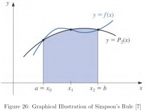
when $n=2$ , the second order Lagrange polynomial is a parabolic curve, and the resulting summation formula involving cubic terms is called the Simpson’s rule.

Then, we conclude this section with a brief introduction of other methods of numerical integration such as undetermined coefficients and composite numerical integration.

Numerical Differentiation

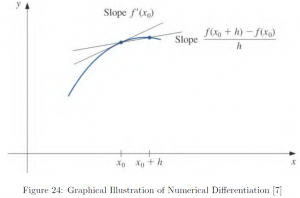
To begin with, let us first revisit the definition of a limit.

$f'(x) = \lim_{h\rightarrow 0} \frac{f(x+h)-f(x)}{h}$

Therefore, for small $h$ , it follows

$f'(x) \approx \frac{f(x+h)-f(x)}{h}$

This is our forward-difference formula. By substituting $h$ with $-h$ , we obtain the backward-difference formula as follows:

$\begin{align*} f'(x) &\approx \frac{f(x-h)-f(x)}{-h}\\ &= \frac{f(x)-f(x-h)}{h} \end{align*}$

Truncation errors can be obtained from the Taylor’s theorem. For $h>0$ , there exists $\xi\in (x,x+h)$ such that

$f(x+h) = f(x) +hf'(x) +\frac{h^2}{2}f''(\xi)$

i.e.

$f'(x) = \frac{f(x+h)-f(x)}{h} - \frac{h}{2}f''(\xi)$

Likewise,

$f'(x) = \frac{f(x)-f(x-h)}{h} + \frac{h}{2}f''(\xi)$

Therefore, the truncation errors for the forward difference-formula and the backward-difference formula are $- \frac{h}{2}f''(\xi)$ and $- \frac{h}{2}f''(\xi)$ , respectively.

Let us illustrate with an example.

Example. Compare the estimates of $\sin'(1)$ with $h=0.1$ , obtained by 2-point forward- and backward-difference formulae.

Let $f(x)=\sin x$ .
Then, $f'(x)=\cos x$

1. Forward-difference estimate

$\begin{align*} \widehat{f'(1)} &= \frac{\sin{(1+0.1)}-\sin{1}}{0.1}\\ &\approx 0.497364 \end{align*}$

2. Backward-difference estimate

$\begin{align*} \widehat{f'(1)} &= \frac{\sin{1}-\sin{(1-0.1)}}{0.1}\\ &\approx 0.581441 \end{align*}$

3. Compare 2 estimates
First, let us compute actual $f'(1)$ .

$\begin{align*} f'(1) &= \cos{1}\\ &\approx 0.540302 \end{align*}$

Therefore, errors are
(a) With forward-difference estimate

$\begin{align*} \varepsilon_F &=\left\vert \widehat{f'(1)}-f'(1) \right\vert\\ &= \left\vert\frac{\sin{(1+0.1)}-\sin{1}}{0.1}-\cos{1} \right\vert\\ &\approx 0.042939 \end{align*}$

(b) With backward-difference estimate

$\begin{align*} \varepsilon_B &=\left\vert \widehat{f'(1)}-f'(1) \right\vert\\ &= \left\vert\frac{\sin{1}-\sin{(1-0.1)}}{0.1}-\cos{1} \right\vert\\ &\approx 0.041138 \end{align*}$

4. Check error bounds
(a) Of forward-difference estimate

$\begin{align*} \left\vert - \frac{h}{2}f''(\xi)\right\vert &= \left\vert -\frac{0.1}{2}\left(-\sin\xi\right)\right\vert\\ &= \left\vert 0.05\sin\xi\right\vert\\ &\leq 0.05\sin{(1.1)}\\ &\approx 0.044560368 \end{align*}$

The actual error is within the error bound

$\varepsilon_F \approx 0.042939 < 0.044560368$

(b) Of backward-difference estimate

$\begin{align*} \left\vert \frac{h}{2}f''(\xi)\right\vert &= \left\vert \frac{0.1}{2}\left(-\sin\xi\right)\right\vert\\ &= \left\vert 0.05\sin\xi\right\vert\\ &\leq 0.05\sin 1\\ &\approx 0.042073549 \end{align*}$

The actual error is within the error bound

$\varepsilon_B \approx 0.041138 < 0.042073549$

We can see both estimates, forward and backward, are similarly off by about 0.04, roughly less than 10% of the actual value of $f'(1)$ .

The 3-point formulae and the truncation term of each can also be obtained by algebraic manipulation of Taylor expansion and Taylor theorem of a function differentiable for at least thrice. We introduce the result as follows:

1. 3-point Midpoint Formula

$f'(x) \approx \frac{f(x+h)-f(x-h)}{2h}$

where

$\varepsilon =-\frac{h^2}{6}f'''(\xi)$

2. 3-point Forward Endpoint Formula

$f'(x) \approx \frac{-3f(x)+4f(x+h)-f(x-2h)}{2h}$

where

$\varepsilon =\frac{h^2}{3}f'''(\xi)$

3. 3-point Backward Endpoint Formula

$f'(x) \approx \frac{3f(x)-4f(x-h)+f(x-2h)}{2h}$

where

$\varepsilon =\frac{h^2}{3}f'''(\xi)$

Note the more accurate estimate, with half of the error bound of the other two, would be obtained with the midpoint formula. Let us examine the accuracy of these formulae by comparing with the estimates obtained by 2-point formulae.

Example. Compare the estimates of $\sin'(1)$ with $h=0.1$ , obtained by 3-point midpoint, forward endpoint, and backward endpoint formulae. Also, discuss the accuracy of these estimates by comparing with the results from 2-point formulae in the previous example.

Let $f(x)=\sin x$ .
Then, $f'(x)=\cos x$

1. 3-point midpoint estimate

$\begin{align*} \widehat{f'(1)} &= \frac{\sin(1+0.1)-f(1-0.1)}{2\cdot 0.1}\\ &\approx 0.539402 \end{align*}$

2. 3-point forward endpoint estimate

$\begin{align*} \widehat{f'(1)} &= \frac{-3\sin(1)+4\sin(1+0.1)-\sin(1-0.2)}{2\cdot 0.1}\\ &\approx 0.541887 \end{align*}$

3. 3-point backward endpoint estimate

$\begin{align*} \widehat{f'(1)} &= \frac{-3\sin(1)+4\sin(1+0.1)-\sin(1-0.2)}{2\cdot 0.1}\\ &\approx 0.542307 \end{align*}$

4. Error computing
We know from our previous example

$f'(1) = \cos{1} \approx 0.540302306$

Therefore, errors are

(a) With midpoint estimate

$\begin{align*} \left\vert \widehat{f'(1)}-f'(1) \right\vert &= \frac{\sin(1+0.1)-f(1-0.1)}{2\cdot 0.1}-\cos{1}\\ &\approx 0.000900 \end{align*}$

(b) With forward endpoint estimate

$\begin{align*} \left\vert \widehat{f'(1)}-f'(1) \right\vert &= \frac{-3\sin(1)+4\sin(1+0.1)-\sin(1-0.2)}{2\cdot 0.1}-\cos{1}\\ &\approx 0.001585 \end{align*}$

(c) With backward endpoint estimate

$\begin{align*} \left\vert \widehat{f'(1)}-f'(1) \right\vert &= \frac{-3\sin(1)+4\sin(1+0.1)-\sin(1-0.2)}{2\cdot 0.1}-\cos{1}\\ &\approx 0.002005 \end{align*}$

1. Comparison of errors

$\begin{array}{c|cc} \text{Method} & \widehat{f'(1)} & \text{Error} \\ \hline \text{2-Point Forward-Difference} & 0.497364 & 0.042939 \\ \text{2-Point Backward-Difference} & 0.581441 & 0.041138 \\ \text{3-Point Midpoint} & 0.539402 & 0.000900 \\ \text{3-Point Forward Endpoint} & 0.541887 & 0.001585 \\ \text{3-Point Backward Endpoint} & 0.542307 & 0.002005 \end{array}$

We can see, on average, the estimates from 3-point formulae are much more accurate than 2-point formulae-based estimates with substantially smaller errors. Indeed, this does not come as a surprise in the light of the notion “the more information we have (about the function), the more accurate, i.e. closer to truth, estimate we can yield.”

However, note that our result is based on the assumption $h$ is small. Suppose we are estimating the tangent of the polynomial $f(x)=x^3$ at $x=1$ with $h=1$ . Then, the estimates we would have obtained are:
(a) 2-point forward-difference

$\begin{align*} \widehat{f'(1)} &= \frac{(1+1)^3-1^3}{1}\\ &= 7 \end{align*}$

(b) 2-point backward-difference

$\begin{align*} \widehat{f'(1)} &= \frac{1^3-(1-1)^3}{1}\\ &= 1 \end{align*}$

(c) 3-point midpoint estimate

$\begin{align*} \widehat{f'(1)} &= \frac{(1+1)^3-(1-1)^3}{2\cdot 1}\\ &= 4 \end{align*}$

We can clearly see that all of the estimates above are grossly discordant with the truth value

$f'(1)=3\cdot 1^2=3$

Numerical Integration

Now we turn our attention to numerical integration. As mentioned in the introduction, there are, in fact, quite many instances, where yielding an explicit form of antiderivative is not possible, or obtaining the integral of a given function with elementary techniques, such as substitution and integration by parts, so far we have covered. Following are such instances:

$P(0\leq Z \leq 1)=\int_0^1 e^{-\frac{z^2}{2}}\,dz$ , where $Z\sim \mathcal{N}(0,1)$
$\int_0^{\frac{\pi}{2}}\sin{(\sin\theta)}\,d\theta$

In the cases like above, we attempt to approximate the given function with the Lagrange polynomial. Then, it becomes a question to construct a polynomial of what order of the given interval with how many nodes. The process is quite similar to computing the Riemann sum, yet the difference is we do not take the number of slices of the interval, denoted $n$ , to infinity as done in calculus, but only limit to a certain number, where our computation power allows.

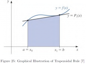
The interpolating polynomial can take the shape of constant, straight line, or parabolic curve, corresponding to the zeroth, first, and second order polynomials. The resultant area under the polynomial is a rectangle, a trapezoid, and an area under a parabolic curve, the organized formula of each is called a rectangular rule, trapezoidal rule, and Simpson’s rule. Note that in the case of the zeroth polynomial, in fact is identical to left Riemann sum.

Let us introduce the Newton-Cotes Formula, the basic form of Lagrange polynomial-based numerical integration.

Theorem. (Newton-Cotes Formula)
Let $P_n(x)$ be the $n$ -th order Lagrange polynomial defined as

$P_n(x) = \sum^n_{i=0}f(x_i)L_i(x) \text{, where } L_i(x) = \prod^n_{k=0,k\neq i}\frac{x-x_k}{x_i-x_k}$

Then,

$\begin{align*} \int_a^b f(x)\,dx &\approx \int_a^b P(x)\,dx\\ &= \int_a^b \sum^n_{i=0} f(x_i)L_i(x) \,dx\\ &= \sum^n_{i=0} f(x_i) \int_a^b L_i(x) \,dx\\ &= \sum^n_{i=0} A_i f(x_i) \end{align*}$

where $A_i = \int_a^b L_i(x) \,dx$ .

Let us consider 3 special cases as follows:
1. Rectangular Rule, where $n=0$
Then,

$\begin{align*} \int_a^b f(x)\,dx &\approx \int_a^b P_0(x)\,dx\\ &= \int_a^b f(a)\,dx\\ &= (b-a)f(a) \end{align*}$

And the truncation error $\varepsilon_R$ is, for $\xi\in (a,b)$ ,

$\begin{align*} \varepsilon_R &= \int_a^b \left(f(x)-P_0(x)\right)\,dx\\ &= \int_a^b f'(\xi)(x-a)\,dx\\ &= f'(\xi)\int_a^b (x-a)\,dx\\ &= \frac{f'(\xi)}{2}(b-a)^2 \end{align*}$

2. Trapezoidal Rule, where $n=1$
Then,

$\begin{align*} \int_a^b f(x)\,dx &\approx \int_a^b P_1(x)\,dx\\ &= \int_a^b \left(f(a)L_0(x)+f(b)L_1(x)\right) \,dx\\ &= \int_a^b \left(f(a)\frac{x-b}{a-b}+f(b)\frac{x-a}{b-a}\right) \,dx\\ &= \frac{b-a}{2}\left(f(a)+f(b)\right) \end{align*}$

And the truncation error $\varepsilon_T$ is, for $\xi\in (a,b)$ ,

$\begin{align*} \varepsilon_T &= \int_a^b \left(f(x)-P_1(x)\right)\,dx\\ &= \int_a^b \frac{f''(\xi)}{2}(x-a)(x-b)\,dx\\ &= \frac{f''(\xi)}{2}\int_a^b (x-a)(x-b)\,dx\\ &= -\frac{f''(\xi)}{12}(b-a)^3 \end{align*}$

3. Simpson’s Rule, where $n=2$
Then,

$\begin{align*} &\int_a^b f(x)\,dx\\ \approx &\int_a^b P_2(x)\,dx\\ = &\int_a^b \left(f(a)L_0(x)+f\left( \frac{a+b}{2}\right) L_1(x)+f(b)L_2(x)\right) \,dx\\ = &\int_a^b \left( f(a) \frac{\left(x-\frac{a+b}{2}\right)(x-b)}{\left( a-\frac{a+b}{2}\right)(a-b)} + f \left( \frac{a+b}{2}\right) \frac{(x-a)(x-b)}{\left( \frac{a+b}{2}-a \right) \left( \frac{a+b}{2}-b \right)}\right)\,dx\\ &+ \int_a^b \left( f(b) \frac{(x-a) \left( x- \frac{a+b}{2} \right) }{(b-a) \left( b- \frac{a+b}{2} \right) } \right)\,dx\\ = &\frac{b-a}{6} \left( f(a)+4f\left(\frac{a+b}{2}\right)+f(b)\right) \end{align*}$

And the truncation error $\varepsilon_S$ is, for $\xi\in (a,b)$ ,

$\begin{align*} \varepsilon_S &= \int_a^b \left(f(x)-P_2(x)\right)\,dx\\ &= \int_a^b \frac{f'''(\xi)}{3!}(x-a)\left(x-\frac{a+b}{2}\right)(x-b)\,dx\\ &= \frac{f'''(\xi)}{3!}\int_a^b (x-a)\left(x-\frac{a+b}{2}\right)(x-b)\,dx\\ &= -\frac{f^{(4)}(\xi)}{90}\left(\frac{b-a}{2}\right)^5 \end{align*}$

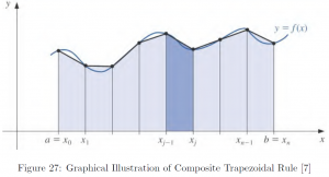
However, rarely is the case we apply the numerical integration rules with only minimal partitions. Suppose we divide the given interval $[a,b]$ into $n$ equally spaced subintervals. Then, we can label the new nodes as

$x_i=a+ih \text{, where } h=\frac{b-a}{n}$

for $i=0,1,2,\cdots,n$ . Then, by applying the trapezoidal or Simpson’s rule over each subinterval and summing them up, they become composite trapezoidal rule and Simpson’s rule, respectively, as follows:

* Composite Trapezoidal Rule

$\int_a^b f(x)\,dx \approx \sum^n_{i=1} \frac{h}{2}\left( f(x_{i-1})+f(x_i)\right)$

Derivation is as follows:

$\begin{align*} \int_a^b f(x)\,dx =& \sum^n_{i=1} \int^{x_i}_{x_{i-1}} f(x)\,dx\\ \approx& \sum^n_{i=1} \frac{h}{2}\left( f(x_{i-1})+f(x_i)\right)\\ =& \frac{h}{2} ( f(x_0)+f(x_1)+f(x_1)+f(x_2)+\cdots\\ &+f(x_{n-2})+f(x_{n-1})+f(x_{n-1})+f(x_n))\\ =& \frac{h}{2} \left( f(a)+2\sum^{n-1}_{i=1} f(x_i)+f(b) \right) \end{align*}$

The truncation error $\varepsilon_T$ for $\xi\in (a,b)$ is

$\begin{align*} \varepsilon_T &= \sum_{i=1}^n \left( -\frac{f''(\xi_i)}{12}h^3\right)\\ &= -\frac{h^3}{12}\sum_{i=1}^n f''(\xi_i)\\ &= -\frac{h^3n}{12}f''(\xi)\\ &= -\frac{h^2(b-a)}{12}f''(\xi) \end{align*}$

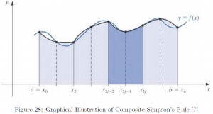
* Composite Simpson’s Rule

$\int_a^b f(x)\,dx \approx \frac{h}{3} \left( f(a) +4\sum^{\frac{n}{2}}_{j=1}f(x_{2j-1}) +2\sum^{\frac{n}{2}-1}_{j=1}f(x_{2j}) +f(b) \right)$

where $n\in 2\mathbb{N}$ .

Derivation is as follows:

$\begin{align*} \int_a^b f(x)\,dx =& \sum^n_{i=1} \int^{x_i}_{x_{i-1}} f(x)\,dx\\ \approx& \sum^n_{i=1} \frac{h}{2}\left( f(x_{i-1})+f(x_i)\right)\\ =& \frac{h}{2} ( f(x_0)+f(x_1)+f(x_1)+f(x_2)+\cdots\\ &+f(x_{n-2})+f(x_{n-1})+f(x_{n-1})+f(x_n))\\ =& \frac{h}{3} \left( f(a) +4\sum^{\frac{n}{2}}_{j=1}f(x_{2j-1}) +2\sum^{\frac{n}{2}-1}_{j=1}f(x_{2j}) +f(b) \right) \end{align*}$

The truncation error $\varepsilon_S$ for $\xi\in (a,b)$ is

$\begin{align*} \varepsilon_S &= \sum_{i=1}^{\frac{n}{2}} \left( -\frac{f^{(4)}(\xi_i)}{90}h^3\right) \left( \frac{x_{2i}-x_{2i-2}}{2}\right)^5\\ &= -\frac{h^5}{90}\sum_{i=1}^{\frac{n}{2}} f^{(4)}(\xi_i)\\ &= -\frac{h^5}{90}\frac{n}{2} f^{(4)}(\xi)\\ &= -\frac{h^4(b-a)}{180} f^{(4)}(\xi) \end{align*}$

Let us conclude this section with an illustrative example.

Example. Estimate $\int_0^{\pi}\sin x \, dx$ using the composite trapezoidal rule and the composite Simpson’s rule, with $n=4$ , and determine error bounds.

In both cases, $h=\frac{\pi}{4}$ , since $n=4$ .

1. Composite Trapezoidal Rule

$\begin{align*} \int_0^{\pi}\sin x \,dx &\approx \frac{h}{2} \left( f(a)+2\sum^{n-1}_{i=1}f(x_i)+f(b) \right)\\ &= \frac{\frac{\pi}{4}}{2} \left( \sin 0+ 2\left( \sin{\frac{\pi}{4}}+\sin{\frac{\pi}{2}}+\sin{\frac{3\pi}{4}}\right) +\sin \pi \right)\\ &= \frac{\pi}{4}(\sqrt{2}+1)\\ &\approx 1.896119 \end{align*}$

2. Composite Simpson’s Rule

$\begin{align*} \int_0^{\pi}\sin x \,dx &\approx \frac{h}{3} \left( f(a) +4\sum^{\frac{n}{2}}_{j=1}f(x_{2j-1}) +2\sum^{\frac{n}{2}-1}_{j=1}f(x_{2j}) +f(b) \right)\\ &= \frac{\frac{\pi}{4}}{3} \left( \sin 0 +4 \left( \sin{\frac{\pi}{4}}+\sin{\frac{3\pi}{4}}\right) +2\sin{\frac{\pi}{2}} +\sin \pi \right)\\ &= \frac{\pi}{6}(2\sqrt{2}+1)\\ &\approx 2.004560 \end{align*}$

3. Error Bounds Determination
The error of approximation using the composite trapezoidal rule is

$\begin{align*} |\varepsilon_T| &= \left\vert -\frac{h^2(b-a)}{12}f''(\xi)\right\vert\\ &= \left\vert-\frac{\left( \frac{\pi}{4}\right)^2 \pi}{12}(-\sin \xi)\right\vert\\ &= \left\vert \frac{\pi^3}{192}\sin \xi \right\vert\\ &\leq \left\vert \frac{\pi^3}{192} \right\vert\\ &\approx 0.161491 \end{align*}$

The error of approximation using the composite Simpson’s rule is

$\begin{align*} |\varepsilon_S| &= \left\vert -\frac{h^4(b-a)}{180}f^{(4)}(\xi)\right\vert\\ &= \left\vert -\frac{\left( \frac{\pi}{4}\right)^4 \pi}{180} \sin \xi\right\vert\\ &= \left\vert \frac{\pi^5}{46080}\sin \xi \right\vert\\ &\leq \left\vert \frac{\pi^5}{46080} \right\vert\\ &\approx 0.006641 \end{align*}$

We confirm the actual errors computed below are within the error bounds.

$\begin{align*} \left\vert \varepsilon_T \right\vert &= \left\vert\widehat{\int_0^{\pi}\sin x \,dx}-\int_0^{\pi}\sin x \,dx \right\vert\\ &\approx 0.103881\\ \left\vert \varepsilon_S \right\vert &= \left\vert\widehat{\int_0^{\pi}\sin x \,dx}-\int_0^{\pi}\sin x \,dx \right\vert\\ &\approx 0.004560 \end{align*}$

Note the error is much smaller when using composite Simpson’s rule than the composite trapezoidal rule. This is in line with our intuitive understanding from the graphical illustration. Indeed, increasing $n$ would result in a smaller error, and taking $n$ to infinity makes it essentially a regular integration.

32 Numerical Calculus

Numerical Differentiation

Numerical Integration

License

Share This Book