One-Variable Equation

Donovan D Chang

30 One-Variable Equation

In this section, we deal with equations with only a single variable, most often denoted by $x$ , either polynomial, non-linear, or mixed functions.

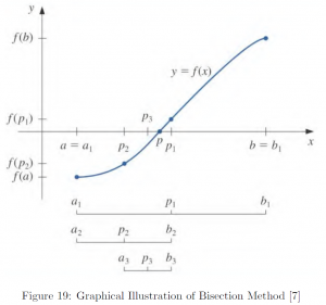
The Bisection Method

The bisection method is arguably the most basic and elementary analytic approach to obtaining solutions. In fact, this is based on the intermediate value theorem discussed in the previous section Analysis, specifically, limits and continuity.

Let us revisit the intermediate value theorem.

Intermediate Value Theorem

Given a continuous function $f:[a,b]\rightarrow \mathbb{R}$ , where $f(a)\neq f(b)$ , the intermediate value theorem} warrants the existence of at least one solution in $c\in (a,b)$ such that $f(c)=k$ , where $\text{min}\left(f(a),f(b)\right)<k<\text{max}\left(f(a),f(b)\right)$ .

Here, we let $k=0$ . Then, the intermediate value theorem becomes $f(a)f(b)<0$ . Let us illustrate the iteration algorithm of bisection method with the second motivating example where $f(x)=\tan x-x$ .

1. Identify 2 points $a$ and $b$ such that $f(a)<0$ and $f(b)>0$ .

$f(4.5) = \tan(4.5)-4.5 \approx 0.1373>0$

Therefore, let $b_1=4.5$ .
Arbitrarily, let us check $f(4.4)$ .

$f(4.4) = \tan(4.5)-4.5 \approx -1.3037<0$

Therefore, let $a_1=4.4$ .

2. Set the first midpoint $p_1=\frac{a_1+b_1}{2}$ .
Then, $p_1=\frac{a_1+b_1}{2}=4.45$ .
Therefore,

$f(p_1) = f(4.45) = \tan(4.45)-4.45 \approx -0.7267<0$

Therefore, let $a_2=4.45$ , and keep $b_2=b_1$ .

3. Continue iteration with $p_n=\frac{a_n+b_n}{2}$ .

if $f(p_n) = \tan(p_n)-p_n =0$ , then we are done with a conclusion $x=p_n$ .
if $f(p_n) = \tan(p_n)-p_n <0$ , then let $a_{n+1}=p_n$ and $b_{n+1}=b_n$ , and continue iteration.
if $f(p_n) = \tan(p_n)-p_n >0$ , then let $a_{n+1}=a_n$ and $b_{n+1}=p_n$ , and continue iteration.

4. Terminate when one of the stopping criteria is met:

$|p_n-p_{n-1}|<\epsilon$
$\frac{|p_n-p_{n-1}|}{|p_n|} <\epsilon$ , where $p_n\neq 0$
$\left\vert f(p_n)\right\vert <\epsilon$

where $\epsilon$ is some small number we set (e.g. $10^{-14}$ ).

Stopping Criterion

There is no right or wrong criteria for stopping. Rather, it actually depends on how much we know about the behavior of $f$ and $p$ . However, if little is known about $f$ and $p$ , then we would be better off by taking the safest or the most conservative approach, (b) $\frac{|p_n-p_{n-1}|}{|p_n|} <\epsilon$ , where $p_n\neq 0$ , since this criterion is closest to testing relative error.[7]

Let us have a look how first ten iterations look. Errors in the last column were defined as $\left\vert \widehat{f(x)}-f(x)\right\vert$ , where $x=4.49340945790906$ , a reasonably accurate estimate of $f(x)=0$ , was assumed to be the solution of $f(x)$ .

$\begin{array}{c|ccccccc} n &a_n &b_n &f(a_n) &f(b_n) & p_n & f(p_n) & \text{Error} \\ \hline 1 &4.4 &4.5 &-1.3037 &0.1373 &4.45 &-0.7267 &0.043410\\ 2 &4.45 &4.5 &-0.7267 &0.1373 &4.475 &-0.3419 &0.018410\\ 3 &4.475 &4.5 &-0.3419 &0.1373 &4.4875 &-0.1161 &0.005910\\ 4 &4.4875 &4.5 &-0.1161 &0.1373 &4.4938 &0.0069 &0.000341\\ 5 &4.4875 &4.4938 &-0.1161 &0.0069 &4.4906 &-0.0555 &0.002784\\ 6 &4.4906 &4.4938 &-0.0555 &0.0069 &4.4922 &-0.0245 &0.001222\\ 7 &4.4922 &4.4938 &-0.0245 &0.0069 &4.4930 &-0.0089 &0.000441\\ 8 &4.4930 &4.4938 &-0.0089 &0.0069 &4.4934 &-0.0010 &0.000050\\ 9 &4.4934 &4.4938 &-0.0010 &0.0069 &4.4936 &0.0029 &0.000145\\ 10 &4.4934 &4.4934 &-0.0010 &0.0029 &4.4935 &0.0010 &0.000048 \end{array}$

We observe a decreasing trend in errors, yet note it only is a trend, but not absolute. In fact, the errors have increased from eighth through tenth iterations, though minimally.

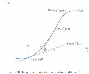
Newton’s Method

Now we turn to the famous Newton’s or Newton-Rhapson method, based on Taylor’s theorem. Owing to its utility and power, naturally this technique has become well-known.

Let us first have a look at Taylor’s theorem.

Theorem. (Taylor’s Theorem [7])
Suppose $f$ is a $n$ -differentiable function $[a,b]$ , denoted $f\in C^n[a,b]$ ; $f^{(n+1)}$ is defined on $[a,b]$ ; and $x_0\in [a,b]$ . Then, for all $x\in [a,b]$ , there exists a number $\xi$ between $x_0$ and $x$ with

$f(x) = P_n(x)+R_n(x),$

where

$P_n(x) = f(x_0) +f'(x_0)(x-x_0) +\frac{f''(x_0)}{2!}(x-x_0)^2 +\cdots+\frac{f^{(n)}(x_0)}{n!}(x-x_0)^n$

and

$R_n(x) = \frac{f^{(n+1)}(\xi)}{(n+1)!}(x-x_0)^{(n+1)}.$

In Taylor’s theorem, $f$ is decomposed into two different functions $P_n(x)$ and $R_n(x)$ , which denote the $n$ -th Taylor polynomial and the remainder term (or truncation error), respectively. By taking $n$ to the limit, we obtain the famous Taylor series and the special case where $x=0$ is called a Maclaurin series.

Note that Taylor’s theorem only ensures the existence of some number $\xi$ in the interval $(a,b)$ , but does not guarantee explicit determination of $\xi$ . Still, the warranted existence of $\xi$ allows us to conduct an error analysis and determine an error bound.

To derive Newton’s method, let us consider the Taylor expansion of $f(x)$ expanded about $p_0$ and evaluated at $x=p$ :

$f(p) = f(p_0) +(p-p_0)f'(p_0) +\frac{(p-p_0)^2}{2!}f''(p_0) +\cdots$

Let $f(p)=0$ , i.e. $p$ is the solution of our interest. Then,

$0 = f(p_0) +(p-p_0)f'(p_0) +\frac{(p-p_0)^2}{2!}f''(p_0) +\cdots$

It is our assumption $|p-p_0|$ is small. Therefore, higher powers of $|p-p_0|$ would be even smaller. Hence,

$0 \approx f(p_0) +(p-p_0)f'(p_0)$

Solving for $p$ , we have

$p \approx p_0 -\frac{f(p_0)}{f'(p_0)}=p_1$

Generalizing for $n\in \mathbb{N}$ iteration,

$p_n = p_{n-1} -\frac{f(p_{n-1})}{f'(p_{n-1})}$

Let us illustrate with an example, where $f(x)=\tan x-x$ . Following is the tabulated result of first four iterations. As in the case of the previous example, errors were defined as $\left\vert f(x)-\widehat{f(x)}\right\vert$ at $x=4.49340945790906$ , a reasonably accurate estimate of $f(x)=0$ .

$\begin{array}{c|cccc} n & p_n & f(p_n) & f'(p_n) & \text{Error} \\ \hline 0 & 4.5\quad\quad\:\, & 0.137332 & 21.504849 & 0.006591 \\ 1 & 4.493614 & 0.004132 & 20.229717 & 0.000204 \\ 2 & 4.493410 & 0.000004 & 20.190766 & 0.000000 \\ 3 & 4.493409 & 0.000000 & 20.190729 & 0.000000 \\ 4 & 4.493409 & 0.000000 & 20.190729 & 0.000000 \end{array}$

Note that how rapidly the error decreases below $10^{-7}$ with only two iterations. One might as well think this might be a coincidence. Therefore, let us run another iteration with $p_0=4.6$ .

$\begin{array}{c|cccc} n & p_n & f(p_n) & f'(p_n) & \text{Error} \\ \hline 0 &4.600000 &4.260175 &78.502699 &0.106591\\ 1 &4.545732 &1.398966 &35.339431 &0.052323\\ 2 &4.506146 &0.273551 &22.845500 &0.012736\\ 3 &4.494172 &0.015444 &20.336636 &0.000762\\ 4 &4.493412 &0.000055 &20.191250 &0.000003\\ 5 &4.493409 &0.000000 &20.190729 &0.000000 \end{array}$

Again, note the rapid reduction in errors. With only five iterations the error went below $10^{-7}$ . In fact, this efficiency in approximation is the basis of the fame and wide applications of the Newton’s method. Comparing with the bisection method based on the same initial value $p_0=4.5$ , where merely a fair at best estimate with an error only under $10^{-4}$ was obtained after ten iterations, the Newton’s method yielded much more accurate estimate with an error under $10^{-6}$ with only two iterations.

So, can we say the Newton’s method has dominance over the bisection method? The answer is no. While the Newton’s method is substantially powerful with many strengths, it is not universally applicable. To begin with, the main limitation of the Newton’s method is $f'(x)$ has to be defined, i.e. the function of interest $f(x)$ has to be differentiable, yet this is not always the case for a continuous function $f(x)$ .

30 One-Variable Equation

The Bisection Method

Newton’s Method

License

Share This Book