26 Row Reduction and Echelon Form
Note that the strategy we used was the sequential elimination of variables to obtain the value of one variable, then plug in the identified value in the equations we have, and so on. Given any consistent set of equations, applying this elimination approach will lead us to the set of answers. However, as the size of the linear system increases with increased number of equations and variables, this elementary algebraic approach would become more prone to error and even inefficient.
Therefore, we developed an algorithm called row reduction, a variant of Gaussian elimination, to first reorganize the system into a triangular shape called echelon form, and then yield solutions in a reduced echelon form. Let us begin.
Definition. (Echelon and Reduced Echelon Matrix)
A rectangular matrix in echelon form has the following properties:
- Non-zero rows always are placed above all-zero rows.
- Leading entry of an upper row is on the left-side columns of the leading entry of a lower row.
- All entries below the any leading entry are zeroes.
Reduced echelon form requires the following in addition:
- The leading entry of non-zero rows is 1.
- Every value in a given column is 0 except the leading entry 1 of non-zero rows.
Let us revisit the example.
Example. Find the echelon and reduced echelon matrix of the given linear system.
For ![]() ,
,
![]()
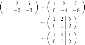
The augmented matrix form of the linear system is

Since we have only 2 equations, with only one row operation we obtained an echelon form,
![]()
The last matrix is in a reduced echelon form, where the values in the last column denote the solutions of the system,
![]()
Inverse and Determinant
Given a matrix equation ![]() , if
, if ![]() is invertible, i.e.
is invertible, i.e. ![]() exists, then we can easily obtain the solution
exists, then we can easily obtain the solution ![]() by
by ![]() .
.
Recall from elementary algebra, for ![]() to be defined,
to be defined, ![]() is a
is a ![]() matrix and its determinant
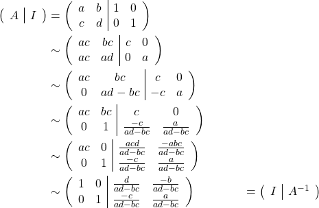
matrix and its determinant ![]() . Here, we demonstrate the notion of determinant naturally arises during the course to obtain the inverse of a
. Here, we demonstrate the notion of determinant naturally arises during the course to obtain the inverse of a ![]() matrix
matrix ![]() . Note that this algorithm is applicable to any
. Note that this algorithm is applicable to any ![]() matrix.
matrix.

Therefore, given ![]() ,
,
![]()
