Vector Spaces

Donovan D Chang

27 Vector Spaces

In the introduction, we discussed the modern understanding of linear systems as vector spaces. To begin with, let us formally define a vector space accompanied with axioms.

Definition. (Vector Space)
A vector space} is a set $V$ upon which the operations, addition} and scalar multiplication} are defined, subject to the following axioms:

For all $\vec{x},\vec{y},\vec{z}\in V$ , and for all scalars $c,d$ ,

$\langle V,+\rangle$ is a group.
$c\vec{x}\in V$
$c(\vec{x}+\vec{y})=c\vec{x}+c\vec{y}$
$(c+d)\vec{x}=c\vec{x}+c\vec{y}$
$c(d\vec{x})=(cd)\vec{x}$
$1\vec{x}=\vec{x}$

Do you get a sense of what a vector space is? In fact, the notion of vector space is quite familiar to us, but we often did not adapt the vector space perspective. Let us think of a 2-dimensional $x$ – $y$ Cartesian coordinate system. It is interesting to see any coordinate $(x,y)\in \mathbb{R} \times \mathbb{R}$ can be seen as a vector space spanned by $\vec{e_x}=\begin{pmatrix} 1\\ 0 \end{pmatrix}$ and $\vec{e_y}=\begin{pmatrix} 0\\ 1 \end{pmatrix}$ . That is,

$\mathbb{R} \times \mathbb{R} = \mathbb{R}^2 = \mathrm{Span}\lbrace \vec{e_x},\vec{e_y}\rbrace =\left\lbrace \begin{pmatrix} x\\ y \end{pmatrix} = x\begin{pmatrix} 1\\ 0 \end{pmatrix} + y\begin{pmatrix} 0\\ 1 \end{pmatrix}: x,y\in \mathbb{R} \right\rbrace$

Euclidean Space $\left(\mathbb{R}^n\right)$

The example we discussed was the $x$ – $y$ Cartesian coordinate system in the light of 2-dimensional vector space, i.e. $\mathbb{R} \times \mathbb{R} = \mathbb{R}^2$ . In fact, this can be expanded to the $x$ – $y$ – $z$ Cartesian coordinate system or a 3-dimensional vector space $\mathbb{R}^3$ , and generalized to $n$ -dimensional vector space $\mathbb{R}^n$ for $n\in \mathbb{N}$ , though not easily visualizable. We call this a Euclidean space. For intuitive exploration, we limit our focus to low-dimensional spaces such as $\mathbb{R}^2$ and $\mathbb{R}^3$ in this summary.

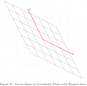
Let us reconsider the example $\mathbb{R} \times \mathbb{R} = \mathbb{R}^2 = \mathrm{Span}\lbrace \vec{e_x},\vec{e_y}\rbrace$ . The vectors in the spanning set coincided with the unit vector on $x$ – and $y$ -axis, respectively. However, it need not be a case. That is, so long as at least two vectors of non-zero magnitude with non-zero angle are included in the set, the set can span the whole $\mathbb{R}^2$ . Let us illustrate with an example.

Example. Show that $\mathbb{R}^2 = \mathrm{Span}\left\lbrace \begin{pmatrix} \cos\theta\\ \sin\theta \end{pmatrix}, \begin{pmatrix} 1\\0 \end{pmatrix}\right\rbrace$ , where $\theta\in (0,\pi)$ .

Expressing $\mathrm{Span}\left\lbrace \begin{pmatrix} \cos\theta\\ \sin\theta \end{pmatrix}, \begin{pmatrix} 1\\0 \end{pmatrix}\right\rbrace$ in a parametric vector form, we have, for all $x,y\in \mathbb{R}$

$x\begin{pmatrix} \cos\theta\\ \sin\theta \end{pmatrix}+ y\begin{pmatrix} 1\\0 \end{pmatrix} = \begin{pmatrix} x\cos\theta +y\\ x\sin\theta \end{pmatrix}$

Let $r\in \mathbb{R}$ , and choose $x=\frac{r}{\sin\theta}$ .
Then, there exists $x=\frac{r}{\sin\theta}$ such that $x\sin\theta=\frac{r}{\sin\theta}\cdot \sin\theta=r\in \mathbb{R}$ .
Therefore, $\mathbb{R}\subseteq \left\lbrace x\sin\theta: x\in \mathbb{R},\theta\in(0,\pi)\right\rbrace$ .

Now, choose $y=-x\cos\theta +r$ .
Then, there exists $y=-x\cos\theta +r$ such that $x\cos\theta+y=x\cos\theta+\left(-x\cos\theta +r\right)=r$ .
Therefore, $\mathbb{R}\subseteq \left\lbrace x\cos\theta +y: x,y\in \mathbb{R},\theta\in(0,\pi)\right\rbrace$ .

We omit the rest of the proof, and conclude $\mathbb{R}^2 = \mathrm{Span}\left\lbrace \begin{pmatrix} \cos\theta\\ \sin\theta \end{pmatrix}, \begin{pmatrix} 1\\0 \end{pmatrix}\right\rbrace$ , where $\theta\in (0,\pi)$ .

Though we have not provided a complete proof, we believe the reader, at least intuitively, saw the possibility of spanning the whole $\mathbb{R}^2$ given 2 vectors of not a scalar multiple of each other. Also, note that the continuity or the completeness axiom of $\mathbb{R}$ is embedded in our proof.

Subspace

Now, we move onto subspace, a subset of a vector space. Formal definition is as follows:

Definition. (Subspace)
Given a vector space $V$ , a subspace $H$ is a subset of $V$ such that

$\vec{0}\in H$
$H$ is closed under addition
$H$ is closed under scalar multiplication

In short, a subspace can be thought of a subset of a vector space containing the origin, denoted by $\vec{0}$ . However, note that a subspace is defined on the space of the same dimension. That is,

$\mathbb{R}^m \not\subset \mathbb{R}^n \text{ for any } m\neq n$

For example, a subset $H=\left\lbrace \begin{pmatrix} x\\y\\0 \end{pmatrix}: x,y\in \mathbb{R} \right\rbrace$ is essentially an $x$ – $y$ plane, yet is defined on $\mathbb{R}^3$ , and thus a subset of $\mathbb{R}^3$ . Again, in fact, $\mathbb{R}^2 \not\subset \mathbb{R}^3$ .

Null Space and Column Space

We shall conclude this chapter introducing 2 other important concepts, null space and column space. In short, a null space is a set of solutions where $\vec{b}=0$ . That is,

Definition. (Null Space)
For a linear system $A\vec{x}=\vec{0}$ , the null space of $A$ is

$\mathrm{Nul}(A) = \left\lbrace \vec{x}:A\vec{x}=0 \right\rbrace$

Column space is another term for a spanned set whose element is every column of a given matrix. That is,

Definition. (Column Space)
The column space of $A= \begin{pmatrix} \vec{c_1} & \vec{c_2} & \cdots & \vec{c_j} \end{pmatrix}$ is

$\mathrm{Col}(A) =\mathrm{Span} \left\lbrace \vec{c_1}, \vec{c_2}, \cdots, \vec{c_j}\right\rbrace$

Let us illustrate with an example.

Example. Identify the column and null spaces of $A= \begin{pmatrix} 2 & 3\\ -2 & 1\\ 1 & -1 \end{pmatrix}$ .

1. $\mathrm{Nul}(A)$
Let us row-reduce the augmented matrix of $A$ . Then,

$\begin{align*} \begin{pmatrix} A & \vec{x} & \vec{0} \end{pmatrix} &= \begin{pmatrix} 2 & 3 & 0\\ -2 & 1 & 0\\ 1 & -1 & 0 \end{pmatrix}\\ &\sim \begin{pmatrix} 2 & 3 & 0\\ 0 & 4 & 0\\ 0 & -\frac{5}{2} & 0 \end{pmatrix}\\ &\sim \begin{pmatrix} 1 & 0 & 0\\ 0 & 1 & 0\\ 0 & 0 & 0 \end{pmatrix}\\ \end{align*}$

Therefore, there only exists a trivial answer $\vec{x}=\vec{0}$ , where $x_1=x_2=0$ .
Therefore,

$\mathrm{Nul}(A) = \vec{0}$

2. $\mathrm{Col}(A)$
By definition,

$\begin{align*} \mathrm{Col}(A) &= \mathrm{Span} \left\lbrace \begin{pmatrix} 2\\-2\\1 \end{pmatrix}, \begin{pmatrix} 3\\1\\-1 \end{pmatrix} \right\rbrace\\ &= \left\lbrace x\begin{pmatrix} 2\\-2\\1 \end{pmatrix} +y\begin{pmatrix} 3\\1\\-1 \end{pmatrix}:x,y\in \mathbb{R} \right\rbrace \end{align*}$

Therefore, $\mathrm{Nul}(A) = \vec{0}$ and $\mathrm{Col}(A) = \left\lbrace x\begin{pmatrix} 2\\-2\\1 \end{pmatrix} +y\begin{pmatrix} 3\\1\\-1 \end{pmatrix}:x,y\in \mathbb{R} \right\rbrace$ .

Note that both $\mathrm{Nul}(A)$ and $\mathrm{Col}(A)$ are subspaces of $\mathbb{R}^j$ , while the null space is implicitly defined, and the column space explicitly. Also, note that $\mathrm{Nul}(A)$ is in fact equivalent to the kernel of the given linear transformation. Recall the definition of kernel is a collection of elements whose image is an identity element in the range, in this case $\vec{0}$ .

27 Vector Spaces

Subspace

Null Space and Column Space

License

Share This Book