Numerical Methods

Donovan D Chang

Numerical Methods

What is numerical analysis or numerical methods? And why do we need it? A brief definition given by Oxford [4] states

“Numerical analysis is the branch of mathematics that deals with
the development and use of numerical methods for solving problems.”

The point here is the use of numerical methods, as opposed to analytic or exact methods, to solve problems, usually expressed in the form of equations. Now we wonder when, i.e. under what circumstances or conditions, would we want to utilize numerical methods. To illustrate, let us look at the following examples.

1. Suppose a pin perfectly fits in a square box whose length of each side is 1 cm. Then, what is the length $l$ of this pin?

We know from the Pythagorean Theorem, the exact answer is

$\sqrt{2} = \sqrt{1^2+1^2} \ \text{cm}$

However, what if we only need a reasonably close estimate of the length to make pins of a similar length with a ruler whose marking is in millimeters (mm)? What we mean by similar in this context is the difference in length with the referent pin is, for example, less than $10^{-4}$ cm, so that in a practical sense the pins appear identical.

It is possible the measurements differ depending on the measurer and the measuring device used. That is,

One might answer $l\approx 1.41$ cm
Another might answer $l\approx 1.414$ cm
Some might answer $l\approx 1.4142$ cm

What do you think is or are correct answers? The answer is it depends. Rather, a more appropriate question would be how accurate these estimates are, or how close these approximations are to the truth value. We shall define an error as the distance of the approximation from the truth value, and denote with $\varepsilon$ ,

$\varepsilon =\left\vert \hat{x}-x\right\vert,$

where $\hat{x}$ denotes an approximation of $x$ .

As all the students answers are approximations, inherently they all contain errors. That is, $\varepsilon\neq 0$ in all cases, i.e.

$l=\sqrt{2}\neq 1.41,1.414,1.4142$

In fact, no matter how many decimal places we obtain by measurements, we know there will be an error, since $\sqrt{2}$ is an irrational number and thus cannot be expressed in fraction or in a finite decimal. Then, would we say they all are wrong and useless? Probably not. Again, depending on the accuracy we need, in other words, depending on the error bound we allow, all of them, some of them, or even none would be found useful.

2. Analyzing diffraction of light from a single-slit experiment, the strength of light has relative maximums at $x=\tan x$ , where $x$ is the distance from the center. Then, how do we identify these points, i.e. solve this equation?

Unfortunately, it is not possible to solve in an analytic and exact manner. Then, what do we do?

Let us first plot the functions, $x$ and $\tan x$ .

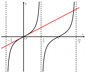
Now, let $f(x)=\tan x-x$ .

We can easily see $f(0)=0$ . Then, let us focus on the solutions in $\mathbb{R}^+$ , since $f$ is an odd function, i.e. $f(x)=-f(-x)$ .

By eye measurements, we see there is a solution, i.e. the two graphs $y=x$ and $y=\tan x$ intersect, at a point in $\left( \pi, \frac{3}{2}\pi\right)$ , but closer to $\frac{3}{2}\pi\approx 4.712$ .

From this point, we use brute force. That is, for guesses $x_i$ ,

if $f(x_i)=0$ , then $x_i$ is a solution.
if $f(x_i)=\tan x_i-x_i<0$ , then try $f(x_j)$ for $x_j\in \left( \pi, \frac{3}{2}\pi\right)$ such that $x_j>x_i$ .
if $f(x_i)=\tan x_i-x_i>0$ , then try $f(x_j)$ for $x_j\in \left( \pi, \frac{3}{2}\pi\right)$ such that $x_j<x_i$ .

Maybe we can begin from $x=4.5$ . Note that the determination of the initial value 4.5 was arbitrarily. That being said, we can begin from any value in $\left( \pi, \frac{3}{2}\pi\right)$ , say, 3.15 or 4. However, in such cases, it will just not be efficient.

$f(4.5)\approx -0.137332055<0$

Therefore, we conclude our next guess should be a value a little bit smaller than 4.5. However, the question of by how much and in what manner afterwards naturally arises. The solution-finding or solution-approximating process is inherently iterative. Therefore, it is of crucial importance to find and apply a more efficient approach. That being said, another way of defining numerical methods is as an organized algorithm to identify close-enough or approximate solutions.

We conclude this motivating example introducing a reasonably accurate estimate of a solution, 4.49340945790906. Again, note this value is not exact and thus indeed technically not a correct answer. Also, note the use of approximation ( $\approx$ ) and equal ( $=$ ) sign.

$\begin{align*} f(4.49340945790906) &= \tan(4.49340945790906)-4.49340945790906\\ &\approx -8.88178\times 10^{-14}\\ &= -0.0000000000000888178\\ &\approx 0 \end{align*}$

In the first motivating example, we illustrated a case where an exact answer can be obtained by an analytic method. Again, we emphasize the only and correct answer is nothing but $\sqrt{2}$ . However, for polynomial equations of higher order, and non-linear equations as seen in the second example, identifying analytic and exact solutions are impossible or extremely difficult.

Therefore, we turn our attention to obtaining reasonably close estimates, or approximations suiting our practical purposes, with keen attention on the range of errors or error bounds. Now, let us study the specifics of numerical methods.

Numerical Methods

License

Share This Book