Outline

• Intro to unsupervised learning – differences between supervised/unsupervised
• Principal Components Analysis (PCA)
• Clustering
  • \(K\)-means (not KNN!)
  • Hierarchical Clustering (dissimilarities)

Supervised vs Unsupervised Learning

• The vast majority, and in fact, essentially all algorithms discussed so far this semester, fall under the umbrella of supervised
  learning
• Supervised learning is the term used when an analyst has a collection of features/covariates/predictors \(x\) and is interested in using these quantities to predict some outcome, \(y\)
• Thus, linear regression, logistic regression, discriminant analysis, KNN, CARTs, Random Forests, Bagging, Boosting, SVMs, etc., have all fallen under this umbrella. We start with a training set containing \(x\) values for samples and their labels \(y\), and wish to develop an algorithm that learns from the training data with the goal of predicting new outcomes (test data) accurately.
• Unsupervised learning is fundamentally different – there are no outcomes (\(y\)) in this case, only \(x\) data, which we use to identify clusters or similarities/dissimilarities among portions of the data.
• In a sense, clustering is used to create previously unknown labels in a dataset – the cluster identifications may denote patient similarities (severe, moderate, no disease) or customer similarities (weekend bingers, nightly watchers, infrequent/sporadic bingers), etc.
• As you’ll see, the analyst must make a unique set of design/method decisions when using clustering (how do we measure dissimilarity?).

Challenges in Unsupervised Learning

• Although there are many methods available for conducting unsupervised learning, we will only cover a select few of them.
• Unsupervised learning tends to be subjective; there’s not a simple goal (most accurate prediction of an outcome in supervised learning, for instance), and it is often unclear at what point one should “stop” the process, as we’ll see with hierarchical clustering and \(K\)-means clustering.
• There is no overarching or universal rule for evaluating the results of an unsupervised, or clustering, analysis—it is more subjective than supervised learning.
• In unsupervised learning, we don’t even know the true answer since there are no outcomes, which makes it very challenging.
• Finally, we often use unsupervised learning as part of exploratory data analysis (EDA), i.e., recall principal components regression (which employs principal component analysis—PCA).

Uses of Unsupervised Learning

• Unsupervised learning can help identify smaller subsets of your sample or population that are inherently similar to or different from one another.
• For instance, consider an eHealth site that offers educational materials, support group sign-ups, easy schedule options, and access to treatment providers through their online portal
  • The company may seek to better understand their customers by:
  1. Determining whether the dimensionality of their behaviors might be reduced, and instead of considering many variables, they could look at a smaller collection of weighted averages
  2. Determining whether use behaviors and frequency are similar within specific subsets of their users
  • This information could be used to better anticipate the future actions of their users or anticipate who might benefit the most from new interventions/programs planned for the near term.
• Unsupervised learning provides methods for grouping users, patients, or other samples that are similar (in some to be determined manner) together.

Principal Components Analysis (PCA)

• As we learned in an earlier lecture (Chapter 6 of ISLR), PCA allows reduction of the dimension of the feature space, i.e. the so-called value of \(p\), or the number of covariates
• The way in which PCA operates has already been explained; find the direction in which the data varies the most, then find the direction (orthogonal to the first direction) in which the data vary the second most, and so on until all \(p\) orthogonal directions are identified, in order from largest variability to smallest.
• When many of the \(p\) variables are moderately or highly correlated with one another, PCA can offer an efficient method for reducing the dimensionality of our problem.
• When conducting PCA (identifying the components from the \(x\) values), there is no \(y\) – in Chapter 6 (Model Selection), we used principal components regression (PCR), in which
  components discovered by PCA were immediately used to predict an outcome \(y\).
• In general, PCA refers ONLY to the process of selecting the orthogonal components from a space of covariates \(x\).

Description of Principal Components

• When we have a large dataset, not necessarily many observations, but many variables/fields/features, it is often difficult to visualize or get a handle on the relationships between these variables.
• Pairwise scatterplots can be used, but often, these variables may only contain a small amount of the overall variability in the data – we might easily miss something with this approach.
• The components are designed to give a lower dimensional representation of the data that still contains a high percentage of the information present (information in terms of variability, essentially).
• These new components can be written (\(k\)th component value for \(i\)th subject):

• Thus, each component value (for the \(i\)th subject) is just a linear combination of their original data values.
• The vector \((\phi_{1k}, \phi_{2k}, \dotsc, \phi_{pk})\) is called the vector of factor loadings for the \(k\)th factor
• In order to assure that our solution is scale invariant with respect to the \(\phi\) coefficients, we constrain their sum of squares to be equal to 1, i.e. \(\sum_{j=1}^p \phi_{jk}^2 = 1\) for all \(k = 1, \dotsc , p\).

Description of the Principal Components

• The principal components can illuminate features or relationships between the variables in the higher dimensional setting.
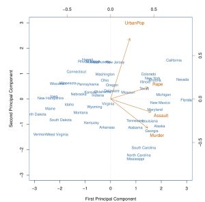
• For example, consider the USArrests data from base R – this data contains four variables for all 50 states in the US – Murder (murder arrests per 100,000), Assault (assault arrests per 100,000),  UrbanPop (percent urban population), and Rape (rape arrests per 100,000).
• As the book shows, PCA can be used to illuminate where most of the information in these features comes from and to determine how these features relate to each other within these components.
• Figure 10.1 shows the relationship between the first and second principal components uncovered from PCA analysis – these components account for approximately 87% of the variability in the variables in the USArrests dataset.
• As can be seen in Figure 10.1, there is a large amount of spread among cities on these two components.
• Also, the variable UrbanPop seems to be weighted lowly in the first principal components but relatively heavily in the second component.

Creating a Biplot for Visualizing the Principal Components

• Figure 10.1 is below:

Notes Regarding the PCA of the Data

• In this example, the number of observations is \(n=50\), and the factor loading vectors are all of length 4 (each new component is a weighted average of the original four variables)
• However, we observe (and you will learn to code this later) that the first two components account for approximately 87% of the variability in the data. Thus, we feel somewhat confident that we can remove the other components and only deal with these two.
• We then find:
  • The first component seems to serve as a sort of proxy for the amount of violent crime that occurred per 100,000 individuals in the cities.
  • The second seems to serve as a proxy for the urban population level and is not as related to the number of violent crimes.
  • This is the extra information that inspecting the biplot yields
• We can further infer, as the book does, that states with low scores for the first component have low violent crime rates, while states with high scores have high violent crime rates, and similarly for the second component.

An Alternative Interpretation

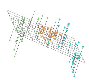
• Another way of looking at the principal components is as follows: since the first principal component finds the direction in which the variability of the feature space is maximized, we can infer that the line (one-dimensional subspace of the feature space) created by this direction is also the line which is closest to the observed data.
• The same can be said for the first two principal components (they form a plane) that are closest to the observed data.
• Figure 10.2a demonstrates this concept in a three-dimensional setting, where the data are simulated.
• Notice that the first two components visualized as a plane (created from their directions) seem to closely approximate the data in three dimensions – the claim is that this is the BEST or closest approximation (to the observed data) possible.
• This is the best two-dimensional representation (a plane) of the data, i.e., it results in a minimum sum of squared distances between data and the solving plane.

An Alternative Interpretation

• Figure 10.2a is below:

The Importance of Scaling

• PCA, as we’ve discussed, finds the direction along which the most variability is observed in the data.
• This means that if one of the variables is measured on a larger scale than the others, which tends to imply a larger variability, then this variable will DOMINATE the amount of variability present in \(x\).
• For this reason, we should be careful to scale variables appropriately when necessary.
• For instance, in the USArrests data, the variances are 18.97, 6945.17, 209.52, and 87.73, respectively for variables Murder, Assault, UrbanPop and Rape.
• This means that the Assault variable may very well overwhelm/dominate the PCA analysis if not scaled appropriately.
• It is important to note that Assault, Murder, and Rape are all measured per 100,000 people, and this number is largely arbitrary. Switching the scale to per 100 would lead to much smaller numbers, and thus, there is little argument for not scaling this data.
• Finally, it is also important to center all data (each feature/covariate around the mean of that feature/covariate) when using PCA – this is done within the function used to conduct PCA.
• NOTE: There may be cases where variables are measured on the same units, i.e., all are rates per 100,000 – then we would not want to scale to SD 1, because all variables are “fairly
  assessed” or “on the same playing field”.

Uniqueness of Principal Components

• In the future, you may notice that when you and another analyst conduct PCA independently, the signs of your loading coefficients and component values may be opposite, i.e., one has positive values, and the other has negative.
• This is not a problem – the directions are still the same, as reflected by the magnitudes of the respective loading coefficients for each factor.
• When \(z_{ij} = \sum_{k=1}^p\phi_{kj}x_{ik}\), this would imply that your \(\phi\) values are the negative of their \(\phi\) values, and your \(z\) values are the negative of theirs. I.e., observing Figure 6.14, the vectors representing the principal components would point in the exact opposite direction. However, this yields the same direction, as the direction is denoted by the line falling along the vector in the x-y plane or higher dimensional space.
• Thus, the principal components are unique, but only up to a sign change – there is no guarantee that separate software packages will yield the same loading coefficients (they may differ by a sign change), or the same components (again, may differ by a sign change) – but this does NOT change the directions representing the components.

Proportion of Variance Explained

• One of the key potential upsides of PCA is the propensity to identify a much smaller number, \(M\), (\(M\) << \(p\)) of components/variables, which are linear combinations of the original \(p\) variables, which account for a large proportion of the variance in \(X\)
• Since PCA projects the original space \(X\) onto a (potentially smaller space) \(Z\), we’d like to know what amount of information is lost
• One can accomplish this by assessing the proportion of variance in \(X\) that is explained by the components \(Z\), which represent the most variability
• Since the \(X\) are centered before analysis, one can represent the total variability in \(X\) by:

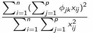
• Now, since \(z_{ik} = \sum_{j=1}^p \phi_{jk}x_{ij}\), the variability in the \(k\)th component is:

• Thus, the percentage of variance explained (PVE) by the \(k\)th component is:

How Many Components?

• Using information gleaned from calculating the PVE for the first series of components, we are tasked with the decision of deciding when “enough of the original variability” has been explained.
• The goal is almost always to reduce the dimensionality of the space- since the first component by definition will account for the most variability, and the second the second most variability, etc., we would like to find the smallest number of components from this set to use without significant loss of information.
• How many components are necessary to still have a “good” understanding?
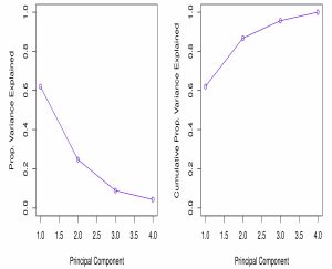
• To answer this, we often use a scree plot, which plots the PVE values for the components identified.
• Figure 10.4 shows a scree plot for the USArrests data – notice that there is an “elbow” between the 2nd and 3rd components. This so-called “elbow” is usually used to determine how many components to include in our dimension reduction analyses.
• The point is, that the 3rd and 4th components explain a small portion (\(\approx 13 \%\)) of the variability, and thus can most likely be discarded.
• Finally, as seen in Chapter 6, one could use \(p\), the number of components to include in regression analysis as a tuning parameter to be selected by CV.

How Many Components?

• See Figure 10.4 below:

Cluster Analysis

• Cluster analysis is distinct from PCA in that, instead of looking for a lower-dimensional characterization of the data, the aim is to identify unknown labels or subgroups in the dataset characterized by similar feature values or similar relationships (correlations) between feature values among individuals in the same cluster, and different feature values are found between clusters.
• Clustering can be used to:
  1. Identify species of flowers in a sample of many distinct species
  2. Identify subtypes of cancer based on patient genetic information
  3. Identify distinct customer behavior profiles in an e-commerce or entertainment site
  4. Identify distinct trading habits in a stock market (or perhaps cryptocurrency) investing application
• We will consider two types of clustering: \(K\)-means, and hierarchical clustering
• \(K\)-means clustering determines the number of clusters up front and then finds the “best” cluster membership for each observation iteratively
• Hierarchical clustering progresses in a “bottom up” fashion (in this lecture, at least), sequentially clustering observations based on their similarity/dissimilarity to other clusters/observations
  • We will discuss a couple of different ways to conduct hierarchical clustering – there are MANY ways to do this in the literature

\(K\)-means Clustering

• In \(K\)-means clustering, we start with the value of \(K\) (analysts often consider multiple values of \(K\) in their analyses)
• The goal is to identify \(K\) clusters, denoted \(C_1, C_2, \dotsc, C_K\), which are mutually exclusive (non-overlapping), and which cover the entire dataset, i.e., each observation belongs to a cluster.
• Written mathematically, this can be denoted:

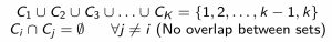
• Thus, if the \(i\)th observation is in cluster \(k\), we write \(i \in C_k\)
• The idea here is to form clusters wherein individual observations are as similar as possible. When all variables are quantitative, we often do this by minimizing the variation within each of the \(K\) clusters, i.e., minimizing the “within cluster variability”
• The solution minimizing the within-cluster variability over all clusters can be written mathematically as:

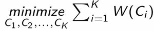
• Where \(W(C_i)\) is the within-cluster variability in cluster \(i\), we want to find \(K\) clusters where the sum of the within-cluster variation over all clusters is minimized.

Finding the \(K\) clusters

• There are many ways that we could define the variation within each cluster, but the most common one has been the squared Euclidean distance:

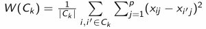
• Here, \(|C_k|\) denotes the number of observations in cluster \(k\), i.e. the number of \(i\) such that \(x_i \in C_k\)
• Essentially, the square of distances for all possible pairs of observations in \(C_k\) is formed and then summed together before dividing by the number of observations in
  \(C_k\)
• Putting this together with the equation on the last slide, we have:

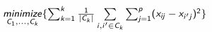
• The question now becomes: how to solve this equation? There are MANY potential solutions, i.e. how many ways can we group n objects into \(K\) clusters. Remember, the sizes of
  each cluster are not constrained, besides having to be \(\leq n – K + 1\) (so that each cluster has at least one observation assigned). However, Algorithm 10.1 provides one solution.

Solving the \(K\)-means Problem

• Algorithm 10.1 below outlines the solution to the \(K\)-means problem:

1. Randomly assign a number from 1 to \(K\) to each observation. These will be the initial assignments for the base case of the iterative
   algorithm.
2. Iterate until the cluster assignments stop changing:
   1. For each of the \(K\) clusters, compute the centroid (multivariate mean). The \(k\)th cluster centroid is then the vector of \(p\) feature means for observations in the \(k\)th cluster.
   2. Assign each observation to the cluster whose centroid is closest to it

• At the end of this algorithm, a local optimum is obtained. Multiple runs should be used with different random starting values in order to determine the best solution. The best solution will be identified by calculating the sum of within-cluster variations over all clusters and selecting the minimum
• The book provides an identity regarding why this algorithm works – essentially, at each run of the algorithm, assigning each observation to the cluster whose centroid is closest will minimize the distance between the observation and the centroid of that cluster, which is equivalent to the definition of within-cluster variation given earlier

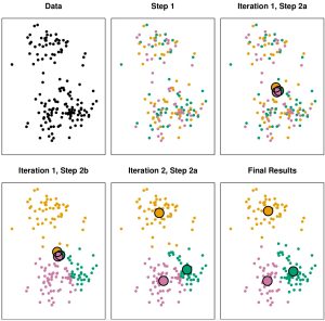
A Visual Example

• Figure 10.6 shows multiple steps (including substeps) of the \(K\)-means algorithm:

Summary

• This lecture discussed in somewhat general terms, the difference between supervised and unsupervised learning (labels or not?)
• Sometimes, we may use unsupervised methods when there are labels (see the example) – the point is, we do not use the labels in the generation of the labels, i.e. \(K\)-means uses no \(y\) data, neither does hierarchical clustering
• Discussed PCA
• Clustering Methods
  • \(K\)-means
  • Hierarchical clustering
• In most cases, you need to pay special attention to scaling issues in clustering. For example, should all units of measure have SD equal to 1?