
3. Learn about GIS database more
Examining Data Properties
We will review each dataset in your current ArcGIS to gain a deeper understanding of its properties, including data source, spatial extent, and spatial reference.
1. In the Contents pane, right-click on US_counties.shp. Then click Properties:

2. Check the Layer Properties: US_counties window:

3. Click Source on the left box. You can find Data source, Extent, Spatial Reference, Domain, Resolution, and Tolerance in the box. These are the primary data information required for geospatial analysis. Click each of them to get information.
4. Here is one of the essential pieces of information you need to focus on. Click Extent:

Stop and Check: The Extent of US_counties displays numbers in the Top, Bottom, Left, and Right, with measurements in meters. The meter is one of the units used in Projected Coordinate Systems (PCS) for GIS and cartography.
5. Let’s check the Spatial Reference of US_roads. Click Spatial Reference
Stop and Check: It shows the Geographic Coordinate System. The Geographic Coordinate System (GCS) is one of the methods used to describe a location on the curved Earth’s surface. We will discuss more Projected/Geographic Coordinate Systems in the next class about “Map Projection.”
Question 2 (1 pt.):
- What is the a) Extent (with the unit) and b) name of the Spatial Reference in the US_counties.shp?
- What is the a) Extent (with the unit) and b) name of the Spatial reference in the US_rivers.shp?
- Based on your answers to the previous two questions, do you notice the differences between these two layers? Explain what these are with two keywords: unit and geographic (or projected) coordinate system.
Explore Attribute Table
In Week 1, we briefly discussed two components of GIS data models: 1) spatial database and 2) attribute. Let’s check the attribute information.
1. In the Contents pane, uncheck all the layers but the US_counties.shp so you can only visualize the county map.
2. In the Contents pane, right-click on US_counties.shp. and click Attribute Table. Then the US_counties table opens:

The attribute table delivers numeric and text information related to the US_counties spatial data by row and column, much like a simple spreadsheet database. Each row of the table corresponds to a part of the feature. Scroll to the right, left, up, and down to browse the attribute data, e.g., state name, county name, census data (P0010001), etc.
Stop and Check: 2020 Census State Redistricting Data (Public Law 94-171) (2020 Census State Redistricting Data (Public Law 94-171) Summary File) provides the Fields and Data dictionary reference name. For example, “P0010001” is a code for Total Population.
3. From the attribute table, you will select counties with a population greater than the average total population in 2020. Right-click on “P0010001” and click Explore Statistics:

4. Write down the “Mean” value of the county-level total population in the chart. And close the statistics window.
5. On the ribbon and in the Table group, click Select By Attributes:

6. Click the drop-down icon next to Where and find “P0010001” (which is the total population), condition (is greater than), and number (put the “Mean” value without a “comma” that you saw in the previous step), like below, by clicking the drop-down icon. Click Run:
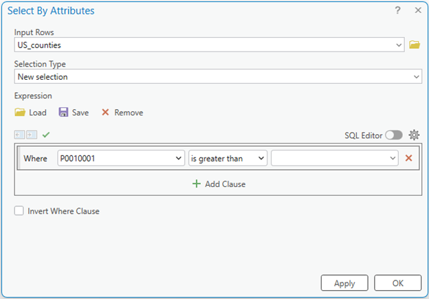
Stop and check: How many rows were selected? (Hint: check the number of “cyan” colored rows presented below the attribute table.)
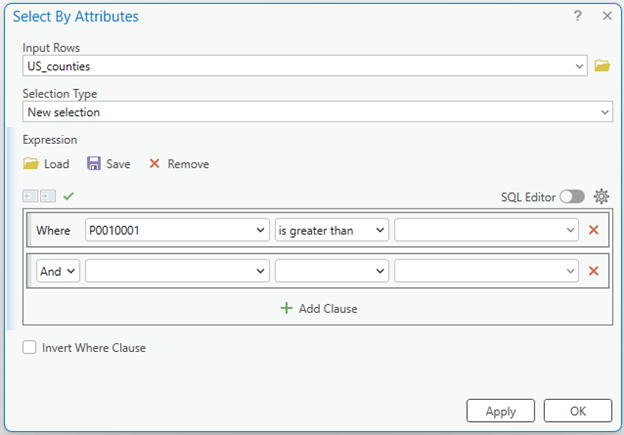
7. Now, add another criterion in step 5. Suppose you want to analyze ethnicity in counties with a Hispanic or Latino population greater than the average county-level population. We will add another criterion to the selected US_counties.shp by:
-
- Finding the “Hispanic or Latino” code in the “HISPANIC OR LATINO, AND NOT HISPANIC OR LATINO BY RACE” item fields in the 2020 Census State Redistricting Data (Public Law 94-171) Summary File
- Re-selecting the counties where the Hispanic or Latino population is more than half of the selected counties.
8. Then click Add Clause and fill in the second clause with your selected census variable, criterion, and value:
Question 3
- How many rows were selected now? (0.2 pts.)
- Make a screenshot of your selected counties and name three regions where the selected counties are clustered. (0.3 pts.)
- What is your interpretation of the final selection? (1 pt.)
Important takeaway: By Questions 5 and 6, you are done with simple query exercises. You will do more table selection and performance-based queries in Week 7
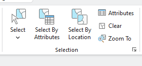
9. You have completed the selection query. Clear existing selection by clicking the Clear button in the Selection tools in the Map tab in the Ribbon:
10. Close the US_counties table by clicking the x icon
11. Save the project