
2 Chapter 2: Linear Models and Systems of Linear Equations
Chapter 1: Linear Models and Systems of Linear Equations
Sections:
1.1 Review of Lines
1.2 Modeling with Linear Functions
1.3 Systems of Two Equations in Two Unknowns
• Exercises
In this chapter we are going to discuss lines, linear models, and systems of linear equations in two variables.
1.1 Review of Lines
Learning Objectives: In this section, you will review concepts of lines, including writing the equation of a line and graphing in the coordinate plane. Upon completion you will be able to:
• Derive an equation of a line given two points or a point and a slope.
• Graph a line, by hand, using any appropriate technique.
• Describe the change in the coordinates of points on a line by applying the definition of slope.
Plotting Ordered Pairs in the Cartesian Coordinate System
An old story describes how seventeenth-century philosopher/mathematician René Descartes invented the system that has become the foundation of algebraic geometry while sick in bed. According to the story, Descartes was staring at a fly crawling on the ceiling when he realized that he could describe the fly’s location in relation to the perpendicular lines formed by the adjacent walls of his room. He viewed the perpendicular lines as horizontal and vertical axes. Further, by dividing each axis into equal unit lengths, Descartes saw that it was possible to locate any object in a two-dimensional plane using just two numbers-the displacement from the horizontal axis and the displacement from the vertical axis.
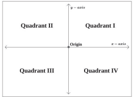
While there is evidence that ideas similar to Descartes’ grid system existed centuries earlier, it was Descartes who introduced the components that comprise the Cartesian coordinate system, a grid system having perpendicular axes. Descartes named the horizontal axis the x-axis and the vertical axis the y-axis. The Cartesian coordinate system, also called the rectangular coordinate system, is based on a two-dimensional plane consisting of the x-axis and the y-axis. Perpendicular to each other, the axes divide the plane into four sections. Each section is called a quadrant; the quadrants are numbered counterclockwise. The center of the plane is the point at which the two axes cross and is known as the origin. (See Figure 1.1.2).
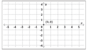
The two axes are similar to number lines, with positive increasing numbers to the right and above the origin and negative decreasing numbers to the left and below the origin. The axes extend to positive and negative infinity as shown by the arrowheads in Figure 1.1.3 below. Each point in the plane is identified first by its x-coordinate, or horizontal displacement from the origin, and second by its y-coordinate, or vertical displacement from the origin. Together, we write them as an ordered pair indicating the combined distance from the origin, (0, 0), in the form (x, y).
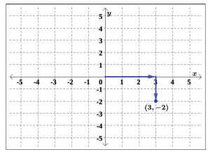
The point (3, −2) is represented in the plane by moving three units to the right of the origin in the horizontal direction, and then two units down in the vertical direction. (See Figure 1.1.4.)
When dividing the axes into equally spaced increments the x-axis may be considered separately from the y-axis. In other words, while the x-axis may be divided and labeled according to consecutive integers, the y-axis may be divided and labeled by increments of 2, or 10, or 100. In fact, the axes may represent specific and different units, such as years against the balance in a savings account, or quantity against cost, and so on. Therefore, it is imperative to label both axes with proper units to convey the meaning of the graph. Consider the rectangular coordinate system primarily as a method for showing the relationship between two quantities.
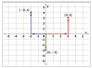
Example 1: Plot the points (−2, 4), (3, 3), and (0, −3) in the coordinate plane.
Solution: To plot the point (−2, 4), begin at the origin. The x-coordinate is -2, so move two units to the left. The y-coordinate is 4, so then move four units up in the positive y direction. To plot the point (3, 3), begin again at the origin. The x-coordinate is 3, so move three units to the right. The y-coordinate is also 3, so then move three units up in the positive y direction.
To plot the point (0, −3), begin again at the origin. The x-coordinate is 0. This tells us not to move in either direction along the x-axis. The y-coordinate is -3, so then move three units down in the negative y direction.
See the points plotted in Figure 1.1.5, below.
When either coordinate of a point is zero, the point must be on an axis. If the x-coordinate is zero, the point is on the y-axis. If the y-coordinate is zero, the point is on the x-axis.
Graphing Linear Equations by Plotting Points
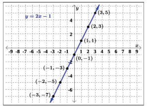
We can plot a set of points to represent an equation. When such an equation contains both an x and a y variable, it is called an equation in two variables; its graph is called a graph in two variables. Any graph on a two-dimensional plane is a graph in two variables. Suppose we want to graph the equation y = 2x − 1. We can begin by substituting a value for x into the equation and determining the resulting value of y. Each pair of x – and y-values is an ordered pair that can be plotted. Table 1.1 lists integer values of x from -3 to 3 and the resulting values for y, when y = 2x − 1.
| x | y = 2x − 1 | (x, y) |
| -3 | y = 2(−3) − 1 = −7 | (−3, −7) |
| -2 | y = 2(−2) − 1 = −5 | (−2, −5) |
| -1 | y = 2(−1) − 1 = −3 | (−1, −3) |
| 0 | y = 2(0) − 1 = −1 | (0, −1) |
| 1 | y = 2(1) − 1 = 1 | (1, 1) |
| 2 | y = 2(2) − 1 = 3 | (2, 3) |
| 3 | y = 2(3) − 1 = 5 | (3, 5) |
Table 1.1: A table of x-values and corresponding y-values for y = 2x − 1.
We can plot the points from the table on the coordinate plane. The selected points for this particular equation appear to form a line, as shown in Figure 1.1.6. While only a few ordered pairs from the equation, y = 2x − 1, were plotted, by connecting these points the line represents all ordered pairs that would satisfy this equation. The arrows on each end of the line indicate there are points outside of the graphed area. Not all equations form a line when the corresponding points are plotted, but we will shortly discuss how to recognize, before plotting points, when the equation will represent a line.
It is important to know that, when plotting points to graph an equation, the x-values chosen are arbitrary, regardless of the type of equation we are graphing. Of course, some situations may require particular values of x to be plotted in order to see a particular characteristic. Otherwise, it is logical to choose values that can be easily calculated with, and it is always a good idea to choose values that are both negative and positive. There is no rule dictating how many points to plot, although we need at least two points to graph a line (a concept that will become clear shortly). Keep in mind, however, that the more points we plot, the more accurately we can sketch the graph.
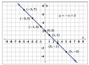
Example 2: Graph the equation y = −x + 2, by plotting points.
Solution: First, choose x-values at random, calculate the corresponding y-values, and construct a table similar to Table 1.1.
| x | y = −x +2 | (x, y) |
| -5 | y = −(−5) + 2 = 7 | (−5, 7) |
| -3 | y = −(−3) + 2 = 5 | (−3, 5) |
| -1 | y = −(−1) + 2 = 3 | (−1, 3) |
| 0 | y = −(0) + 2 = 2 | (0, 2) |
| 1 | y = −(1) + 2 = 1 | (1, 1) |
| 3 | y = −(3) + 2 = −1 | (3, −1) |
| 5 | y = −(5) + 2 = −3 | (5, −3) |
Table 1.2: A table of x-values and corresponding y-values for y = −x + 2.
Now, we plot the points and connect them to see they form a line, as shown in Figure 1.1.7.
Try It 0
Construct a table and graph the equation y = 12x + 2, by plotting points.
Writing a Linear Equation
Thus far, we have discussed techniques for graphing a line given its equation. Now we will turn our attention to representing a line algebraically by writing the equation which describes the relationship between the x – and corresponding y-values.
When writing the equation of a line, we describe both its “steepness” and the set of points that define the line.
Slope: To get a sense of the “steepness” of a line, we compute the slope of the line by simply using any two ordered pairs on the line and the formula below.
Definition 1.0
The slope, m, of the line containing the points P (x1, y1) and Q (x2, y2) is given by
m = y2 − y1
x2 − x1
= Δy
Δx = change in y
change in x
provided x1 = x2
Note that:
When x1 = x2, the slope of the line between the two points P and Q is undefined.
When y1 = y2, the slope of the line between the two points P and Q is 0.
A couple of comments about the above definition are in order. First, don’t ask why we use the letter “m” to represent slope; there are many explanations out there, but apparently no one really knows for sure. Secondly, the stipulation x1 =/ x2 ensures that we aren’t trying to divide by zero. The reader is invited to pause and think about what is happening geometrically.
Example 3: Compute the slope of the line that passes through the points (2, −1) and (−5, 3).
Solution: Let (x1, y1) = (2, −1) and (x2, y2) = (−5, 3). Then, we can substitute the y-values and the x-values into the slope formula, as follows.
m = y2 − y1
x2 − x1
m = 3 − (−1)
−5 − 2
= 4
−7
= −4
The slope of the line through the given points is −4/7 .
It does not matter which point is called (x1, y1) or (x2, y2). As long as we are consistent with the order of the y-terms and the order of the x-terms in the numerator and denominator, the calculation will yield the same result.
m = y2 − y1
x2 − x1
= y1 − y2
x1 − x2
Try It 1
Compute the slope of the line that passes through the points (2, 3) and (2.1, 4).
Whether we are given the coordinates of two points on a line, as ordered pairs, or only given a visual representation of the line, we can still determine the slope of the line using the slope formula.
Example 4: Using Figure 1.1.13, determine the slope of each line: A, B, C, and D.
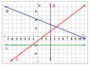
Figure 1.1.13: The graph of four different lines.
Solution: We can compute the slope of each line by selecting any two points on the line. Consider- ing we can choose any two points, we will choose points with “nice” integer coordinates.
A. For line A, we can identify two points: (0, −2) and (6, −2). The slope can then be computed using the formula.
m = −2 − (−2)
6 − 0
= −2+2
6
= 0
6
= 0
B. For line B, we can identify two points: (0, 4) and (10, 0). The slope can then be computed using the formula.
m = 0 − 4
10 − 0
= −4
10
= −2
5
C. For line C, we can identify two points: (−4, −4) and (0, −1). The slope can then be computed using the formula.
m = −1 − (−4)
0 − (−4)
= −1+4
0+4
= 3
D. For line D, we can identify two points: (3, −2) and (3, 0). Notice x1 = x2, which would also be true for any two points on line D. Thus, by the definition, the slope of line D is undefined.
If we would have substituted the coordinates of the two points, (3, −2) and (3, 0), into the slope formula, the result would have included a denominator of zero. Because we cannot divide by zero, we would have again concluded the slope of line D is undefined.
If the slope of a line is positive (as with line C), the line slants to the right. This means positive (negative) changes in x result in positive (negative) changes in y. If the slope of a line is negative (as with line B), the line slants to the left. This means positive (negative) changes in x result in negative (positive) changes in y. If the slope of a line is zero (as with line A), the line has no slant and is horizontal. If the slope of a line is undefined (as with line D), the line again has no slant, but is vertical.
Horizontal and Vertical Lines
Notice in the previous example that every point on the horizontal line (line A) has the same y-coordinate. In general, the y-coordinate of every point on a horizontal line is the same, b. Therefore, the common equation of a horizontal line is y = b.
Then notice again in the previous example that every point on the vertical line (line D) has the same x-coordinate. In general, the x-coordinate of every point on a vertical line is the same, a. Therefore, the common equation of a vertical line is x = a.
Definition 1.1
- The equation of a horizontal line through the point (a, b) is y = b.
- The equation of a vertical line through the point (a, b) is x = a.
The x-axis is the horizontal line y = 0, and the y-axis is the vertical line x = 0.
Example 5: Write the equation of line A and line D, from the previous example.
Solution: Line A is horizontal, and every point on the line has a y-coordinate of -2. Thus, the equation of line A is y = −2.
Line D is vertical, and every point on the line has an x-coordinate of 3. Thus, the equation of line D is x = 3.
Point-Slope Form
We have discussed the equations of vertical and horizontal lines. Using the concept of slope, we can develop equations for the other varieties of lines. Suppose a line has a slope of m and contains the point (x1, y1). Let (x, y) be an arbitrary point on the line, as indicated in Figure 1.1.14.
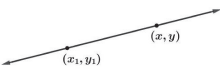
The slope between these two points yields
m = y − y1
x − x1
m (x − x1) = y − y1
y − y1 = m (x − x1)
After manipulating the slope formula, we have just derived one form of the equation of a line, known as the point-slope form of a line.
Definition 1.2
The point-slope form of the line, with slope m and containing the point is the equation.
When using the point-slope form of the line, any point on the line can be used to determine the equation. If done correctly, equivalent equations will be obtained.
Example 6: Write the equation of the line with slope m = −3 and passing through the point (4, 8), using the point-slope form of a line.
Solution: Using the point-slope form, substitute -3 for m and the point (4, 8) for (x1, y1).
y − y1 = m (x − x1)
y − 8 = −3(x − 4)
Example 7: Write the equation of the line containing the points (−1, 3) and (2, 1), using the point- slope form of a line.
Solution: First, we need to determine the slope of the line in question. Using the given points and slope formula, we have
m = Δy
Δx
= 1 − 3
2 − (−1)
= −2
3
We can use either point in the point-slope form, but we’ll use (−1, 3) as (x1, y1) and leave it to the reader to check that using (2, 1) results in an equivalent equation. Substituting into the point-slope form of the line, we get
y − y1 = m (x − x1)
y − 3 = −2
3
(x − (−1))
y − 3 = −2
3
(x + 1)
Recall that slope can be described as the ratio change in y . We found the slope in the previous example to be −2 = −2 . We can interpret this as a change in y of 2 units downward for every 3 unit change in x to the right, as we travel along the line to the right. This interpretation is shown in the graph of the line, y − 3 = −2 (x + 1), in Figure 1.1.15 below. (Notice both of the given points are on the line.)
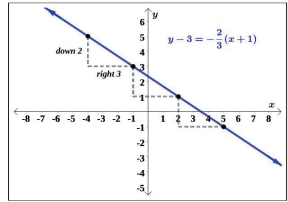
Mathematically the slope −2 = −2 is also equal to 2 , the slope can also be interpreted as a 3 3 −3 2 units increase of y for every 3 units decrease in x, as you travel along the line to the left.
Slope-Intercept Form
We can further simplify the equation of the line in the previous example, to produce another form of a line called the slope-intercept form. This is the familiar y = mx + b form you have probably seen in algebra. The “intercept” in the slope-intercept form comes from the fact that if we set x = 0, we get y = b. This point, (0, b), is the y-intercept of the line y = mx + b. Intercepts of a line will be discussed in more detail later in this section.
Definition 1.3
The slope-intercept form of the line, with slope m and y-intercept (0, b) is the equation
When using the slope-intercept form of a line, if we have slope m = 0, we get the equation y = b which matches our formula for a horizontal line. The slope-intercept form of a line can be used to describe all lines except vertical lines.
Further simplification of the resulting line in the previous example gives us
y − 3 = −2
3
(x + 1)
y − 3 = −2
3
x − 2
3
y = −2
3
x +
7
3
In this format, y = mx + b, we can verify the slope of the line is m = −2 , and we now know the y-intercept of the line is (0, 7 ). 3
Example 8: Write the equation of the line passing through the points (3, 4) and (0, −3), using slope-intercept form.
Solution: First, we calculate the slope using the slope formula and the given two points.
m = −3 − 4
0 − 3
= −7
−3
= 7
3
Next, we use the point-slope form with the slope of 7 , and either point. Let’s pick the point (3, 4) for (x1, y1).
y − 4 = 7
3
(x − 3)
To write the equation in slope-intercept form, we start by distributing the 7 , and then simplify.
y − 4 = 7
3
x − 7
y = 7
3
x − 3
In slope-intercept form, the equation of the line is written as y = 7 x − 3.
To prove that either point can be used, when using the point-slope form, let us use the second point, (0, -3), and show that we get the same the equation in slope-intercept form.
y − (−3) = 7
3
(x − 0)
y +3= 7
3
x
y = 7
3
We see that the same line will be obtained using either point. This makes sense because we used both points to calculate the slope.
Also, notice we were given the y-intercept, (0, −3), as our second point. We could have skipped substitution into the point-slope form and substituted directly into the slope-intercept form of a line.
Try It 2
Write the equation of the line passing through the points (2,3) and (2.1, 4) in both point-slope form and slope-intercept form.
Standard Form
Another way that we can represent the equation of a line is in standard form.
Definition 1.4
The standard form of a line is given as Ax+By=C, where A, B, and C are integers.
When a line is written in standard form, the x – and y-terms are on one side of the equals sign and the constant term is on the other side.
Example 9: Write the equation of the line with a slope of -6 which passes through the point ( 1 , −2) in standard form.
Solution: We begin by using the point-slope form of a line.
y − (−2) = −6 (x − 1/4 )
We next simplify to the slope-intercept form of a line.
y +2= −6x +
3
2
y = −6x − 1
2
We can then rearrange terms and multiply both sides of the equation by 2, the least common denominator, to obtain integers coefficients and an integer constant term.
6x + y = −1
2
12x + 2y = −1
This equation is now written in standard form, 12x + 2y = −1.
There are different situations where one form of a line is preferred over the others for practical or computational purposes, and there are also times where any of the forms is perfectly reasonable to use. Throughout this course you will see each form and its usefulness.
Finding x-intercepts and y-intercepts
Previously, the y-intercept of a line was mentioned in our discussion of the slope-intercept form of a line. In general, the intercepts of any graph, including that of a line, are the points at which the graph intersects (i.e., crosses/touches) the axes.
Definition 1.5
• The y-intercept is the point at which the graph intersects the y-axis and has coordinates (0, y).
• An x-intercept is a point at which the graph intersects the x-axis and has coordinates (x, 0).
To determine a y-intercept, we set x equal to zero and solve for y. Similarly, to determine an x-intercept, we set y equal to zero and solve for x. In the case of lines, there will be at most one y-intercept. For example, let’s determine the intercepts of the line 12x + 2y = −1 from the previous example.
To solve for the y-intercept, set x = 0.
12x + 2y = −1
12(0) + 2y = −1
2y = −1
y = −1
2
0, −1
2
is the y-intercept
To solve for the x-intercept, set y = 0.
12x + 2y = −1
12x + 2(0) = −1
12x = −1
x = − 1
12
− 1
12, 0
is the x-intercept
The intercepts are easily identifiable points that can be used to graph a line.
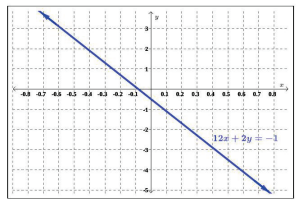
We can confirm that our results make sense by observing a graph of 12x +2y = −1, as shown in Figure 1.1.16. Notice the graph crosses the axes where we predicted it would.
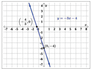
Example 10: State the intercepts of the line y = −3x − 4. Then, sketch a graph of the line, using only the intercepts.
Solution: Set x = 0 to solve for the y-intercept.
y = −3x − 4
y = −3(0) − 4
y = −4
(0, −4) is the y-intercept Set y = 0 to solve for the x-intercept.
y = −3x − 4 0 = −3x − 4
4 = −3x
4
− = x 3/ 4− , 03)is the x-intercept
To sketch a graph of the line, plot both intercepts on the coordinate plane, and draw a line passing through them, as in Figure 1.1.17.
Another method for graphing a line, using a known point on the line and the slope of the line, is to plot the point and use the understanding of slope in terms of “change in y” and “change in x.” Starting at the given point, move the appropriate number of units up/down and then right/left, according to the slope, to plot another point on the line. You can now draw your line through the two points.
Interpreting Slope
Given the line y = −11 x + 17, if we know x increases by 3 units as you move along the line, how can we find the corresponding change in y? As the slope of the line is negative, we know the graph of the line will slant to the left and that a positive change in x (increase) should produce a negative change in y (decrease). From its definition, we know slope can be written as
Δy
m =
Δx
which shows the constant relationship between changes in the x-coordinates of points on a line and changes in the y-coordinates of points on a line.
From the given equation we have m = −11 = Δy . If x increases by 3 units, then Δx = 3.
Using substitution we have
11 Δy
− =
8 3
Through multiplication and simplification we can find the corresponding change in y, Δy.
−11(3) = 8(Δy)
−33 = 8(Δy)
33
− = Δy 8
Thus, y decreases by 33 units when x increases by 3 units.
When the change in a variable is negative, this corresponds to a decrease in the variable value, while a positive change corresponds to an increase in the variable value.
Example 11: You have a line which passes through the points (2, −1) and (−5, 3).
(a) If x decreases by 9 units, what is the corresponding change in y?
(b) If y increases by 5 units, what is the corresponding change in x?
Solution: First, we calculate the slope using the slope formula with the given two points.
m = Δy
Δx
= 3 − (−1)
−5 − 2
= 4
−7
= −4
7
Because the slope is negative, we should recognize that an increase in one variable will produce a decrease in the other and vice versa.
(a) If x decreases by 9 units, then Δx = −9. So,
4 Δy
m = − =
7 −9
Through multiplication and simplification we can find the corresponding change in y.
−4(−9) = 7(Δy)
36 = 7(Δy)
36
= Δy
7
Thus, y increases by 36 units when x decreases by 9 units.
(b) If y increases by 5 units, then Δy = 5. So,
4 5
m = − =
7 Δx
Through multiplication and simplification we can find the corresponding change in x, Δx.
−4(Δx) = 7(5)
−4(Δx) = 35
Δx = 35
−4
Δx = −35
4
Thus, x decreases by 35 units when y increases by 5 units.
Watch your signs when simplifying fractions. For example, −a = −a = a but −a =/ −a .
b b −b b −b
Try It 3
Given the line −7x + 3y = −9, if y decreases by 2 units, what is the corresponding change in x?
Try It Answers
-
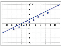
- A table of points and corresponding graph are given below.
| x | y = 1 x +2
2 |
(x, y) |
| -8 | -2 | A = (−8, −2) |
| -6 | -1 | B = (−6, −1) |
| -4 | 0 | C = (−4, 0) |
| -2 | 1 | D = (−2, 1) |
| 0 | 2 | E = (0, 2) |
| 2 | 3 | F = (2, 3) |
| 4 | 4 | G = (4, 4) |
| 6 | 5 | H = (6, 5) |
2. m = 10
3. Point-Slope Form: y − 3 = 10(x − 2) or y − 4 = 10(x − 2.1)
Slope-Intercept Form: y = 10x − 17
4.
|
x decreases by 6 units
Exercises
Basic Skills Practice
For Exercises 1 − 4, determine the slope of the line passing through the given points.
1. (0,0) and (3,5) 3. y = −3x +6
2. (6,1) and (9,11) 4. 3x − 2y = 6
For Exercises 5 – 8, determine the x – and y-intercept, without graphing. Write each intercept as an ordered pair.
5. y = 5x − 14 7. (5, 0) and (0, −8)
6. 4x + 8y = 9 8. (3, −5) and (−7, −4)
For Exercises 9 – 12, write the equation of the line with the given slope which passes through the given point, in both point-slope form and slope-intercept form, if possible.
9. m = 3 and (3, −1) 11. m = 2 and (−2, 1)
10. m = −2 and (−5, 8) 12. m = −1 and (10, 4)
13. (−3, 10) and (5, −6) 15. (1, 3) and (5, 5)
14. (−6, −15) and (−2, −7) 16. (4, −9) and (−14, 20)
For Exercises 17 – 21, graph the line, without the use of technology, using the given infor- mation.
17. The line has a slope of m = 4/7 and 19. y − 5 = 2 (x − 8)
passes through the origin. 20. y = 7
18. y = −3x +2 21. x = −2
For Exercise 22, describe the changes in x or y, using the given information.
22. Given a line has a slope of m = 3/4,
(a) If x increases by 4 units, what is the corresponding change in y?
(b) If y increases by 3 units, what is the corresponding change in x?
(c) If x decreases by 4 units, what is the corresponding change in y?
(d) If y decreases by 3 units, what is the corresponding change in x?
Intermediate Skills Practice
For Exercises 23 – 26, determine the slope of the line passing through the given points.
23.
|
|
|
|
( 1 , 3 ) and ( 5 , −7 ).
24.
|
|
( 11 , 7) and (−11 , −4).
25. (−1, −2) and (3, −2).
26. (8, 1) and (8, 2).
For Exercises 27 – 30, determine the x – and y-intercept without graphing.
27. 4y = −2x − 1 29. 4x − 3 = 2y
28. 21 − 6y = 7x 30. 2x = 5y − 8
For Exercises 31 – 34, write the equation of the line with the given slope which passes through the given point, in both point-slope form and slope-intercept form, if possible.
31. m = 0 and (3, 117) 33. m is undefined and (10, 6)
32. m = 1.75 and (−4, 8) 34. m = −0.1 and (0.2, 0.9)
For Exercises 35 – 37, write the equation of the line which passes through the given points.
35. (1, 7) and (3, 7) 37. (4, −1) and a y-intercept of (0, 2)
36. (−6, 10) and (−6, 16) 38. (−2, 6) and an x-intercept of (1, 0)
For exercises 39-43, graph the line, without the use of technology, using the given information.
39. y = 2(x + 1) − 4
40.
|
y = 1 (x − 3) + 1
41.
|
y +7 = 4 (x + 2)
42. The line has a slope of zero and passes through the point (−5, 3).
43. The line has an undefined slope and passes through the point (−3, −4).
For Exercise 44, describe the changes in x or y, using the given information.
44. Given the line y = −9/7 x − 1,
• If x increases by 1 unit, what is the corresponding change in y?
• If y increases by 3 units, what is the corresponding change in x?
• If x decreases by 10 units, what is the corresponding change in y?
• If y decreases by 1 unit, what is the corresponding change in x?
Mastery Practice
45. Determine the slope of the line passing through the points (a, −5) and (4, 2a), in terms of a. For what value(s) of a is the slope of the line undefined?
46. Determine the slope, y-intercept and x-intercept, if any exist, for y = 1−x.
47. Write the equation of the line with a slope of 6 which passes through the point (c −5, −4), in point-slope and slope-intercept form, where c is any real number.
48. Write the equation of the line which intersects the x-axis when x = −10 and intersects the y-axis when y = 7
49. Graph the line 5x − 7y = 70, by finding and using the x – and y-intercepts.
50. Given the line 6x + 11y = 19,
(a) If x increases by 1 unit, what is the corresponding change in y?
(b) If y increases by 6 units, what is the corresponding change in x?
(c) If x decreases by 7 units, what is the corresponding change in y?
(d) If y decreases by 11 units, what is the corresponding change in x?
51. If when x decreases by 9 units, y decreases by 2 units, what is the slope of the line containing any point (x, y)?
Communication Practice
52. Describe, in your own words, what the y-intercept of a line is.
53. Describe the process for finding the x-intercept and y-intercept of a line, algebraically.
54. If a point is located on the y-axis, what is the x-coordinate and why does it have this value?
55. If a point is located on the x-axis, what is the y-coordinate and why does it have this value?
1.2 Modeling with Linear Functions

Josh is hoping to get an A in his college math class. He has scores of 75, 82, 95, 91, and 94 on his first five exams. Only the final exam remains, and the maximum number of points that can be earned is 100. Is it possible for Josh to end the course with an A, if all exams are weighted equally? A simple linear equation will give Josh his answer.
Many real-world applications we come across every day can be modeled by linear equations. For example, a cell phone package may include a monthly service fee plus a charge per minute of talk-time; it costs a widget manufacturer a certain amount to produce x widgets per month plus monthly operating costs; a car rental company charges a daily fee plus an amount per mile driven.
Learning Objectives: In this section, you will learn about concepts related to linear depreciation, cost, revenue, profit, supply, and demand. Upon completion you will be able to:
- Formulate the equation for a linear depreciation, cost, revenue, profit, supply, and demand function.
- Solve problems involving linear depreciation, including the rate of depreciation, initial value, and scrap value.
- Describe the relationships between the cost, revenue, and profit functions, graphically and verbally.
- Describe the differences between a supply and demand function.
Defining a Linear Function
The natural world is full of relationships between quantities that change. When we see these relationships, it is natural for us to ask “If I know one quantity, can I then determine the other?” This establishes the idea of an input quantity, or independent variable, and a corresponding output quantity, or dependent variable. From this we get the notion of a functional relationship in which the output can be determined from the input.
For some quantities, like height and age, there are certainly relationships between these quantities. Given a specific person and their age, it is easy enough to determine their height. A function is a rule for a relationship between an input, or independent, quantity and an output, or dependent, quantity in which each input value uniquely determines one output value. We say “the output is a function of the input.”
To simplify writing out expressions and equations involving functions, an algebraic notation is often used. We also use descriptive variables to help us remember the meaning of the quantities in the problem.
Rather than write “height is a function of age,” we could use the descriptive variables h to represent height, a to represent age, and if we name the function f we could then write:
“h is f of a” or h = f (a)
We could instead name the function h and more simply write:
h(a)
For example, consider a 20-year old who is 5 feet 7 inches tall. Then according to our notation, we say
h = f (20) = 5 feet 7 inches or
h(20) = 5 feet 7 inches
The notation h(a) is read “h of a”. Remember we can use any variable to name the function; the notation h(a) shows us that h depends on a. The value ‘a’ must be put into the function ‘h’ to get a result. Be careful when reading function notation.
Warning! Do not confuse the parentheses in function notation with multiplication! In the last scenario, the parentheses indicate that age is input into the function.
For any function,
– The set of all values which can be put into the function is known as the domain of the function.
– The resulting outputs from the function are known as the range of the function.
Definition 1.6
A linear function is a function whose graph produces a line. Linear functions can always be written in the form
f(x) = mx + b or f(x) = b + mx (they’re equivalent)
where b is the initial or starting value of the function (when input, x, is zero), and m is the constant rate of change of the function.
Modeling With Linear Functions
A linear model is a linear function that helps explain real-world scenarios involving quanti- ties changing linearly. Because we are modeling real-world applications, we use descriptive variables appropriate for the scenario, rather than the standard x and y discussed in the pre- vious section. Due to this change, the independent variable values will replace the x-values on the horizontal axis, while the dependent variable values will replace the y-values on the vertical axis. Also, when looking at linear models, domain constraints will be dependent on the problem.
For the purposes of this text, we will focus on economic and business scenarios such as depreciation, cost, revenue, profit, supply, and demand.
Linear Depreciation
Defintion 1.7
Linear depreciation models the loss in value of an asset over time. It can be represented by
V (t) = mt + b
where V represents the value of the asset at time t, b represents the initial value of the asset, and m represents the constant rate of change in value of the asset with respect to time, ΔV
Δt .
A general graph of a linear depreciation function is given below in Figure 1.2.2.
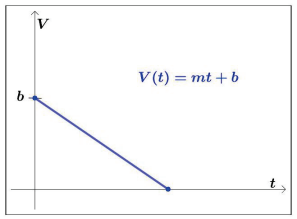
Here, we will restrict our discussion to situations where the value of the asset decreases (depreciates) linearly over time. Thus, the slope of a linear depreciation model should always be negative.
Example 1: A company purchased $120, 000 of new office equipment and expects the value of the equipment to depreciate by $16, 000 per year.
(a) Construct a linear model for the value of the equipment as a function of time.
(b) What is the rate of depreciation of the equipment?
(c) Compute and interpret the horizontal intercept.
(d) Determine a reasonable domain and range for this function.
Solution: (a) In the problem, there are two changing quantities: time and value. The remaining value of the equipment depends on how long the company has owned it. We can start by defining our variables, including units.
Let the outputs, V , and inputs, t, be defined as follows:
V := the value of the equipment, in dollars
t := the time, in years, since purchase
Reading the problem, we identify two important values. The first, $120, 000, is the initial value for V (the value of b in a linear depreciation model). The other value, $16, 000 per year, appears to be a rate of change the units of dollars per year match the units of our output variable divided by our input variable. The value of the equipment is depreciating, so we know that the value remaining is decreasing each year and the rate of change will produce a negative slope (the value of m in a linear depreciation model).
Using the information provided in the problem, we can write the following linear depreciation model:
V (t) = −16000t + 120000
(b) The slope represents the rate of change in value with respect to time, and is equal to – 16000 in this problem, which represents a loss of $16, 000 per year. By definition the slope of a linear depreciation model will always be negative, so the rate of depreciation is the rate at which the value decreases and is defined to be |m|, with units included. Thus, the rate of depreciation for the equipment is $16, 000/ year.
(c) Here the horizontal intercept is the t-intercept, as t is the independent variable. To solve for the t-intercept, we set the dependent variable, V , to zero, and solve for t :
0 = −16000t + 120000
t = 120000
16000
t = 7.5
The horizontal intercept is (7.5, 0); this represents the input value where the output will be zero. Interpreting this, we could say: “The equipment will be worth $0, or will have no remaining value, after 7.5 years.”
(d) When modeling any real-world scenario with functions, there is typically a limited domain over which the model will be valid – almost no trend continues indefinitely. In this problem, it certainly doesn’t make sense to talk about input values less than zero. This model is also not valid after the horizontal intercept, as it does not make sense to talk about the equipment having a negative value.
Domain represents the set of input values. The reasonable domain for this function is 0 ≤ t ≤ 7.5. Range represents the set of output values; the value starts at $120, 000 and ends with $0 after 7.5 years. So, the corresponding range is 0 ≤ V (t) ≤ 120, 000. Most importantly remember that domain and range are tied together, and whatever you decide is most appropriate for the domain (the independent variable) will dictate the requirements for the range (the dependent variable).
In the previous example, we discussed the rate of depreciation and the restricted domain. Related formal definitions can be found below.
Definition 1.8
Rate of depreciation is the amount of value an asset loses per time unit. It can be represented by |m|, with specified units.
Definition 1.9
Scrap value is the lowest value an asset obtains. Once an asset reaches scrap value, it remains at that value indefinitely.
The scrap value is assumed to be zero, unless given other information regarding the actual scrap value or the time when scrap value is reached. In the previous example, the horizontal intercept is (7.5, 0), which means the equipment has no value after 7.5 years. This signifies the scrap value is $0, and it occurs after 7.5 years.
Try It 1
A refrigerator has a value (in dollars) given by V (t) = −400t+5000, where t represents the number of years since the refrigerator was purchased. Determine and interpret
- The rate of depreciation.
- V (0) and V (3)
- The amount of time before the refrigerator reaches scrap value.
In the previous example, we were given the initial value and rate of depreciation. Oftentimes, this is not the case, but instead you may be given different, yet sufficient, information to determine the linear model. In the next example, we will demonstrate how to use skills learned about lines in the previous section to construct a linear model.
Example 2: A new phone is purchased for $839 and is worth $543 two years later. Assuming the value of the phone decreases at a constant rate, answer the following.
(a) Determine the value (in dollars) of the phone, V , as a function of the number of years since its purchase, t.
(b) Determine the value of the phone after 18 months.
(c) If the scrap value of the phone is $10, what is the phone worth after 15 years?
Solution: (a) Because the value of the phone decreases at a constant rate, we are trying to find a linear function of the form
V (t) = mt + b
From the information given, we know that (0, 839) and (2, 543) are two points defined by the function. Thus,
m = ΔV
Δt
= 543 − 839
2 − 0
= −296
2
m = −148
The purchase value of $839 not only gives us the point (0, 839), but also tells us that b = 839. Therefore,
V (t) = −148t + 839
(b) In our function, t represents the amount of years since the phone was purchased. Due to the fact that there are 12 months in 1 year, then
18months = 18months
12 months
year
= 1.5years
Thus, the value after 18 months can be found by evaluating our function when
t = 1.5.
V (1.5) = −148(1.5) + 839
= 617
So, after 18 months, the phone is worth $617.
(c) First, we need to determine how long it takes the phone to reach a scrap value of $10. To do this we set the value, V , equal to 10 and solve for t:
10 = −148t + 839
148t = 829
t = 829
148
t ≈ 5.6years
As the scrap value is the lowest value an item obtains, at any time after approx- imately 5.6 years, the phone will have a value of $10. Thus, after 15 years the phone is still worth $10.
The actual value at time t may differ from the calculated function value at time t, V (t), for any time after an item reaches scrap value. Here, if we compute V (15) = −148(15) + 839 = −1381, we see the actual value, $10, and the function value, −$1381, differ greatly. Notice that, in the context of our problem, it is not possible for the phone to have a value of negative $1381. This would mean that instead of someone paying $10 for the phone after 15 years, you would have to pay them $1381 to take the phone from you.
Cost, Revenue, and Profit
Businesses must keep track of and manage their expenditures, their sales, and the profits they realize. In this text, we will first examine what happens if these transactions are linear in nature.
Definition 1.10
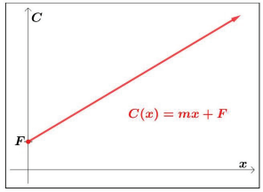
When a company produces x items, the total cost function, C(x), models the total cost of producing those items. The total cost includes both fixed costs, which are startup costs (like equipment and buildings), and variable costs, which are costs that depend on the number of items produced (like materials and labor). In the most simple case,
Total Cost = (Variable Costs)+(Fixed Costs)
= (production cost per item)(quantity)+(fixed costs)
C(x) = mx + F,
where x is the number of items (quantity) produced.
A general graph of a linear total cost function is given below in Figure 1.2.3. Notice that even when 0 items are produced, the company still has fixed costs of $F .
Example 3: It costs a company a total of $1900 to manufacture 60 items, and the company has fixed costs of $700. If x represents the number of items manufactured, write the company’s linear total cost function.
Solution: We are looking for a function of the form C(x) = mx + F . From the information given, we know that (60,1900) and (0, 700) are two points defined by the function. Thus,
m = ΔC
Δx
= 700 − 1900
0 − 60
= −1200
−60
m = 20
With the fixed costs being $700, the linear total cost function then becomes C(x) = 20x + 700
It is important to remember that total costs include both variable and fixed costs. Thus, it is not correct to divide total costs by quantity to obtain the slope. In the previous example, m =/1900/60.
Definition 1.11
Revenue, R(x), is the amount of money a company brings in from sales. In the most simple case,
Revenue = (price per item)(quantity)
R(x) = px,
where x is the number of items (quantity) sold.
A general graph of a linear revenue function is given below in Figure 1.2.4. Notice that when 0 items are sold, the company brings in $0 of revenue.
Figure 1.2.4: The first quadrant of the coordinate plane with a line sloping in the upward direction, starting from the origin.
Example 4: What is the revenue function from selling the items in the previous example, if each item sells for $35?
Solution: By definition revenue is found by multiplying price per item times quantity sold, so we have
R(x) = p · x = 35x
where x represents the number of items sold.
Definition 1.12
Profit, P(x), is the amount of money a company brings in, after expenses.
Profit = Revenue − Total Cost
P(x) = R(x) − C(x),
where x is the number of items (quantity) made and sold.
A general graph of a linear profit function is given below in Figure 1.2.5. Notice that when 0 items are produced and sold, the company will take a loss, due to the fixed costs.
Figure 1.2.5: The first quadrant of the coordinate plane with a line sloping in the upward direction. The line starts on the P -axis at (0, −F ).
Example 5: What is the profit function for the manufacturing and selling of the items produced in the previous examples?
Solution:
P (x) = R(x) − C(x)
= 35x − (20x + 700)
= 35x − 20x − 700
P (x) = 15x − 700
Always subtract ALL costs; remember to distribute the negative. In the previous example, P (x) /= 35x − 20x + 700
When modeling a cost, revenue, or profit function of a company, we must use the appropriate information. At times this requires us to differentiate between types of costs to the company and money received by the company.
Example 6: To manufacture 100 items, it costs a company a total of $32, 000, and to manufacture 200 of these items, it costs the company a total of $40, 000. If each of these items sells for $150, determine the profit function for the company making and selling these items. (Assume linear cost and revenue functions.)
Solution: To determine the company’s profit function, we first need to find the cost and revenue functions. For total cost, we have the points (100, 32000) and (200, 40000) defined by the function. We can now calculate the slope:
m = ΔC
Δx
= 40000 − 32000
200 − 100
= 8000
100
m = 80
Then, using the point (100, 32000) and the point-slope form of a line, C − C1 = m (x − x1), we get
C − 32000 = 80(x − 100)
C − 32000 = 80x − 8000
C(x) = 80x + 24000
Because each item sells for $150, the revenue function is given by R(x) = 150x. There- fore, the profit function will be
P (x) = R(x) − C(x)
= 150x − (80x + 24000)
= 150x − 80x − 24000
P (x) = 70x − 24000
Previously we mentioned that domain constraints of linear models are dependent on the scenario being modeled. As shown in the general graphs of cost, revenue, and profit, the domain of each of these functions is restricted to non-negative values, as x always represents a quantity of items. One could logically say “it is not possible to produce/sell a negative number of items.”
Try It 2
A donut shop estimates their fixed daily expenses are $600. If each donut costs about $0.05 to make and sells for $0.60, determine the shop’s daily total cost, revenue, and profit functions. Then, sketch all three functions on the same graph.
Supply and Demand
In economics, there are models for how prices are determined in a free market which state that supply and demand for a product are related to price. For the purposes of this text, we will assume supply and demand are linear.
Definition 1.13
Demand, D(x), shows the relationship between the quantity of a certain product consumers desire and the price, p, they are willing to pay per item. Typically, as the number of items a consumer needs to purchase increases, the price the consumer is willing to pay per item decreases.
D(x) = price
D(x) = p
or
p(x) = mx + b,
where x is the number of items purchased.
A general graph of a linear demand function is given below in Figure 1.2.6. In the graph, the x-intercept represents the maximum number of items taken by consumers, if the item is free. Moreover, the p-intercept represents the price above which the item will not be purchased by consumers.
Figure 1.2.6: The first quadrant of the coordinate plane with a line segment sloping in the downward direction. The line segment starts on the p-axis at (0, b) and ends when it reaches the x-axis. Due to consumers’ purchasing habits, all linear demand functions will have a negative slope.
Example 7: It has been determined that at a price of $2 a store can sell 2400 of a particular type of toy doll, and for a price of $8 the store can sell 600 such dolls. Determine the price of a doll, p, as a linear function of the number of dolls demanded, x.
Solution: We are trying to find a demand function, D(x), of the form p(x) = mx + b. With the information given, we have the points (2400, 2) and (600, 8) defined by the function.
Calculating the slope:
m = Δp
Δx
= 8 − 2
600 − 2400
= 6
−1800
m = − 1300
Then, using the point (2400, 2) and the point-slope form of a line: p − p1 = m (x − x1), we have demand of
p − 2 = − 1300(x − 2400)
p − 2 = − 1300x + 8
p(x) = − 1300x + 10
We can double check our demand function by substituting the other given point,
(x, p) = (600, 8).
8 ?= − 1300(600) + 10
8 ?= −2 + 10
8=8
Definition 1.14
Supply, S(x), shows the relationship between the quantity of a certain product produc ers are willing to supply based on the price per item, p, that is being offered. Typically, the more items a producer has to sell, the higher the price the producer desires to sell each item.S(x) = price
S(x) = p
or
p(x) = mx + b,
where x is the number of items being sold.
A general graph of a linear supply function is given below in Figure 1.2.7. In the graph, the p-intercept represents the price below which no items will be supplied to the market.
Figure 1.2.7: The first quadrant of the coordinate plane with a line sloping in the upward direction, starting on the p-axis at (0, b). Due to producers wanting the most money possible for the sale of their product, all linear supply functions will have a positive slope.
Example 8: A manufacturer of toy dolls can supply 3000 dolls if the dolls are sold for $8 each, but can supply only 1000 dolls if the dolls are sold for $4 each. Determine the price per doll, p, as a linear function of the number of dolls supplied, x.
Solution: We are trying to find a function of the form p(x) = mx + b. With the information given, we have the points (3000, 8) and (1000, 4) defined by the function. Calculating the slope:
m = Δp
Δx
= 4 − 8
1000 − 3000
= −4
−2000
m = 1500
Then, using the point (3000, 8) and the point-slope form of a line, we have supply of
p − 8 =1500(x − 3000)
p − 8 =1500x − 6
p(x) = 1500x + 2
Often we want to study both supply and demand simultaneously to compare the desires of both the consumers and producers.
Example 9: At a price of $2.50 per gallon, there is a demand in a certain town for 42.5 thousand gallons of gas and a supply of 20 thousand gallons. At a price of $3.50, there is demand for 25.5 thousand gallons and a supply of 28 thousand gallons. Determine the linear supply and demand functions.
Solution: We will use price, p (in dollars), as the output and quantity, x (in thousands of gallons of gas), as the input for both functions. For supply, we have the points (20, 2.50) and (28, 3.50) defined by the function.
Calculating the slope:
m = Δp
Δx
= 3.50 − 2.50
28 − 20
= 18
m = 0.125
Then, using the point (20, 2.50) and the point-slope form of a line,
p − 2.50 = 0.125(x − 20)
p − 2.5=0.125x − 2.5
p(x)=0.125x (Supply)
For demand, we have the points (42.5, 2.50) and (25.5, 3.50) defined by the function. Calculating the slope:
m = Δp
Δx
= 3.50 − 2.50
25.5 − 42.5
= 1−17
m = − 117
Then, using the point (42.5, 2.50) and the point-slope form of a line,
p − 2.50 = − 117(x − 42.5)
p − 2.5 = − 117x + 2.5
p(x) = − 117x + 5
Try It 3
At a price of $3, consumers will purchase 600 mechanical pencils. For every 50 cent decrease in price, consumers will purchase an additional 75 pencils. Determine the linear demand function, p(x).
Try It 4
The producers of mechanical pencils will not supply pencils to the market if the price is below $1, but for every 25 cent increase above $1 the producers will supply an additional 25 pencils. Determine the linear supply function, p(x).
Try It Answers
- (a) The rate of depreciation equals $400/ year ⇒ the refrigerator’s value decreases by $400 each year.
(b) V (0) = 5000 ⇒ The refrigerator is initially worth $5000.
V (3) = 3800 ⇒ After 3 years, the refrigerator is worth $3800.
(c) 12.5 years ⇒ After 12.5 years, the refrigerator has no value. Moreover, at any point in time after 12.5 years, the refrigerator will continue to have zero value.
2. Cost: C(x) = 0.05x + 600,x := the number of donuts produced Revenue: R(x) = 0.60x, x := the number of donuts sold
Profit: P (x) = 0.55x − 600,x := the number of donuts made and sold.
3.
|
p(x) = − 1 x + 7, where x := the number of pencils demanded, and p := the price of a pencil (in dollars).
4.
|
p(x) = 1 x + 1, where x := the number of pencils supplied, and p := the price of a pencil (in dollars).
Exercises
Basic Skills Practice
Writing a linear depreciation function.
1. An item is worth $500 when it is purchased. After 3 years, it is worth $320. Assuming the item is depreciating linearly with time, write the value of the item (in dollars) as a function of time (in years since purchase).
2. An item is bought and 7 years later is worth $1000. The same item is worth $200 fifteen years after purchase. Assuming the item is depreciating linearly with time, write the value of the item (in dollars) as a function of time (in years since purchase).
3. An item purchased for $850 reaches scrap value after 8 years. Assuming the item is depreciating linearly with time, write the value of the item (in dollars) as a function of time (in years since purchase).
For Exercises 4 − 8, the value of an item is given to be V (t) = −25t + 1250, where t is the number of years since the item was purchased and V is given in dollars.
4. What was the purchase price of the item?
5. After how many years will the item be worth only $1000 ?
6. After how many years will the item achieve scrap value?
7. What was the item worth after 30 years?
8. What is rate of depreciation?
Writing a linear total cost, revenue, or profit function.
9. A company has monthly fixed costs of $10, 000 and a production cost of $25 for each item it produces. What is the company’s monthly linear total cost function?
10. A company sells an item it produces to the public for $150 each. What is the company’s linear revenue function?
11. A company has a total cost function of C(x) = 5x + 800 and revenue function of R(x) = 22x. What is the company’s profit function? Linear supply and demand functions.
12.
|
Given a demand function of p(x) = −1 x + 40, where x represents the number of items demanded and p(x) represents the price/item (in dollars),
(a) At what price will 50 items be demanded?
(b) Above what price will consumers not buy this item?
(c) How many items will consumers demand if the items are priced at $20?
(d) How many items will consumers demand if the items are free?
13. Given a supply function of p(x) = 3x + 15, where x represents the number of items supplied and p(x) represents the price/item (in dollars),
(a) At what price will producers supply 100 items to the market?
(b) Producers will only supply the items if the price is above what value?
(c) How many items will producers provide to the market at a price of $45?
Writing a linear supply or demand function.
14. At a price of $20 per item, 100 items are demanded by consumers, but at a price of $50 per item, only 20 items are demanded. Construct the linear demand function, p(x), for this item.
15. At a price of $40 per item, producers will provide 125 items to the market. At a price of
$80 per item, producers will provide 325 items. Construct the linear supply function,
p(x), for this item.
Intermediate Skills Practice
Writing a linear depreciation function.
16. An item is worth $10 when it is purchased. After 10 years, it is worth 50 cents. Assuming the item is depreciating linearly with time, write the value of the item (in dollars) as a function of time (in years since purchase).
17. An item is purchased in 1996 for $400, 000 and in 2010 it is worth $120, 000. Assuming the item is depreciating linearly with time, write the value of the item (in dollars) as a function of time (in years since 1996).
18. An item purchased for $3500 has a scrap value of $200 after 11 years. Assuming the item is depreciating linearly with time, write the value of the item (in dollars) as a function of time (in years since purchase).
For Exercises 19 − 23, the value of an item is given to be V (t) = −85000t + 1000000, where
t is the number of years since the item was purchased and V is given in dollars.
19. What was the purchase price of the item?
20. How many years will it take the item to reach a scrap value of $150, 000?
21. What was the item worth after 5 years?
22. What is the value of the item after 12 years?
23. What is rate of depreciation?
Writing a linear total cost, revenue, or profit function.
24. A company has fixed costs of $15, 000 each month and production costs of $1/ item. If each of these items is sold to the public for $5, determine the company’s monthly linear profit function.
25. A company can produce 20 items for a total cost of $795. If the company has fixed costs of $495, determine the company’s linear total cost function.
26. A company has production costs of $20 per item. If the company can produce 100 items for a total cost of $2850, determine the company’s linear cost function.
27. A company brings in a total of $1275 in revenue from selling 85 items. What is the company’s linear revenue function?
Writing a linear supply or demand function.
28. Consumers will demand 500 items at a price of $2/ item. For every $2 increase in price per item, 4 fewer items will be demanded. Construct the linear demand function, p(x), for this item.
29. Consumers will demand 1000 items at a price of $3.50 per item. When the price per item increases to $4, the number of items demanded will decrease by 50. Construct the linear demand function, p(x), for this item.
30. Producers will supply 50 items at a price of $10 per item. For every $5 increase in price per item, 500 more items will be provided. Construct the linear supply function, p(x), for this item.
31. A producer will not supply any items when the price is $475 or lower, but when the price per item is $500, the producer is willing to supply 800 items. Construct the linear supply function, p(x), for this item.
32. Consumers will buy 8000 items at a price of $20/ item. If the price goes up to $25/ item, they they will only buy 6000 items. Manufacturers will not market this item below
$10, but for every $5 increase in price per item, 2000 more items will be provided to the market.
(a) Construct the linear demand function, p(x).
(b) Construct the linear supply function, p(x).
Mastery Practice
33. An item is bought and after 2 years has a value $5000. Ten years after its purchase, the item is worth $4500. Assuming the item is depreciating linearly, what was the purchase price of the item?
34. An item purchased for $500 has a scrap value of $150 after 14 years. Compute the value of the item after 36 months, assuming the item depreciates linearly. 35. Given the graph below, identify the total cost function, C(x), the revenue function, R(x), and the profit function, P (x).
36. A company finds the total cost of producing 30 items is $9150, while they can produce 55 items for a total cost of $10, 775. Each of these items is sold to the public for $80.
(a) Compute the production cost per item.
(b) Write the company’s linear profit function.
37. A manufacturer has fixed costs of $180 and a production cost of $30 per item manu- factured. What is the selling price of the item, if the company has a profit of $4320 when selling 100 items? (Assume total cost and revenue are linear.)
38. Given x represents the number of items supplied or demanded each month, p represents the unit price of the items (in dollars), Equation A is −5x + 2p = 60 and Equation B is 3x + 2p = 300, answer the following.
(a) Which equation is the demand equation? Why?
(b) How many items will consumers purchase if the items are free?
(c) Above what price will consumers not buy the item?
(d) Producers will only provide the items if the price is above what value?
Communication Practice
- Explain, in your own words, the meaning of the rate of depreciation.
- If a linear depreciation function, V (t), is given for 0 ≤ t ≤ 20, explain how you determine the value of the item for values of t > 20.
- Illustrate the relationships between linear total cost, revenue, and profit functions, graphically.
- Explain, in your own words, why the linear supply function p(x) has a positive slope.
- Explain, in your own words, why the linear demand function p(x) has a negative slope.
Media Attributions
- quadrant
- 1.1.3
- 1.1.4
- 1.1.5
- 1.1.6
- 1.1.7
- 1.1.13
- 1.1.14
- 1.1.15
- 1.1.16
- 1.1.17
- try it 1
- math
- 1.2.2
- 1.2.3