
1
5.1 Relations and Functions
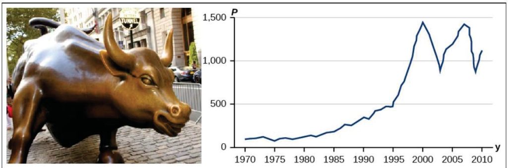
Toward the end of the twentieth century, the values of stocks of internet and technology companies rose dramatically. As a result, the Standard and Poor’s stock market average rose as well. Figure 5.1.1 tracks the value of an initial investment of just under $100 over the 40 years (1970 – 2010). It shows that an investment that was worth less than $500 until about 1995, skyrocketed up to about $1500 by the beginning of 2000. That five-year period became known as the “dot-com bubble,” because so many internet startups were formed. As bubbles tend to do, though, the dot-com bubble eventually burst. Many companies grew too fast and then suddenly went out of business. The result caused the sharp decline represented on the graph, beginning at the end of 2000.
Notice, as we consider this example, that there is a definite relationship between the year and the stock market average. For any year we choose, we can determine the corresponding value of the stock market average.
Learning Objectives: In this section, you will learn about the relationship between rela- tions and functions. Upon completion you will be able to:
- Translate between a set of real numbers and interval notation.
- State whether or not a relation is a function.
- State the domain and range of a given graphical representation of a function, using interval notation.
- Use and apply function notation to given scenarios.
5.2 Writing Interval Notation
We will focus on the use of the real numbers, R. Recall that we may visualize R as a line. Segments of this line are called intervals of numbers, which can be discussed symbolically or graphically. Symbolically, these segments can be written using set-builder or interval notation.
Definition 5.0
- Set-builder notation is a method of specifying a set of elements that satisfy a certain condition. It takes the form {x | statement about x} which is read as, “the set of all x such that the statement about x is true.” For example,
{x | 4 < x ≤ 12}
would be read as “the set of all x such that four is less than x is less than or equal to 12.”
- Interval notation is a way of describing sets that include all real numbers between a lower limit, that may or may not be included, and an upper limit, that may or may not be included. The endpoint values are listed, separated by a comma, between brackets or parentheses. A square bracket, “[” or “]”, indicates inclusion in the set, and a parenthesis, “(” or “)”, indicates exclusion from the set. The example given in set-builder notation above would be written, using interval notation, as
(4, 12]
Graphically speaking, for intervals with finite endpoints, we use a filled-in or ’closed’ dot to indicate an endpoint is included in the interval. On the other hand, an ‘open’ circle is used to signal an endpoint is not included in the interval.
If the interval does not have finite endpoints, we use the symbol −∞ to indicate that the interval extends indefinitely to the left and ∞ to indicate that the interval extends indefinitely to the right. As infinity is a concept, and not a number, when using these symbols we always use parentheses in interval notation, and when graphing we use an appropriate arrow to indicate that the interval extends indefinitely in one (or both) direction(s).
Below is a summary of the different ways to express given sets of numbers.
| Set-Builder
Notation |
Interval
Notation |
Verbal
Description |
| {x | a < x < b} | (a, b) | x is strictly between a and b |
| {x | a ≤ x < b} | [a, b) | x is between a and b and includes a |
| {x | a < x ≤ b} | (a, b] | x is between a and b and includes b |
| {x | a ≤ x ≤ b} | [a, b] | x is between a and b, including a and b |
| {x | x < b} | (−∞, b) | x is less than b |
| {x | x ≤ b} | (−∞, b] | x is less than or equal to b |
| {x | x > a} | (a, ∞) | x is greater than a |
| {x | x ≥ a} | [a, ∞) | x is greater than or equal to a |
| {x | −∞ < x < ∞} | (−∞, ∞) | x is any real number |
Table 5.1: Equivalent Notations for the Description of an Interval
Example 1: Consider the sets of real numbers described in Table 5.2 below. Fill in the missing cells of the table with the different equivalencies.
| Set-Builder Notation | Interval Notation | Verbal Description | |
| a. | x is between -1 and 4, and includes both -1 and 4 | ||
| b. | {x | x ≤ 5} | ||
| c. | (−2, ∞) |
Table 5.2: A table of intervals with missing equivalencies.
Solution:
(a) The given verbal description of the interval is “x is between -1 and 4, and includes both
-1 and 4.” If we break down the statement and start with “x is between -1 and 4,” we get −1 < x < 4. Additionally, the interval “includes both -1 and 4,” so the set-builder notation is {x | −1 ≤ x ≤ 4}. The corresponding segment of the real number line, shown in Figure 5.1.2, starts with a ‘closed’ dot at -1 and ends with a ‘closed’ dot at
4.
![A number line extending from negative infinity to positive infinity. Two solid dots mark the points -1 and 4, with a horizontal line segment connecting them. This represents the closed interval [-1, 4], indicating that all numbers between -1 and 4, including the endpoints, are included.](https://iu.pressbooks.pub/app/uploads/sites/2011/2025/02/image2-2-300x40.jpeg)
Because -1 and 4 are both included, the interval notation is [−1, 4].
(b) The given set-builder notation shows that x must satisfy the inequality x ≤ 5. So, the corresponding segment of the real number line, shown in Figure 5.1.3, extends to −∞ indicated by an arrow to the left and ends with a ‘closed’ dot at 5.
![A number line extending from negative infinity to positive infinity. A solid dot marks the point 5, with a horizontal line extending leftward from 5 toward negative infinity. This represents the interval ( − ∞ , 5 ] (−∞,5], indicating all numbers less than or equal to 5.](https://iu.pressbooks.pub/app/uploads/sites/2011/2025/02/image3-2-300x39.png)
Due to the fact that the real number line extends indefinitely to the left and has a ‘closed’ dot at 5, the corresponding interval notation is (−∞, 5]. The verbal description is “x is less than or equal to 5.”
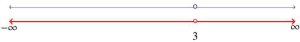
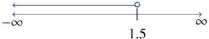
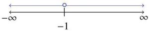
(c) The given interval notation is (−2, ∞), which includes all real numbers greater than -2. The equivalent set-builder notation is {x | x > −2}. The corresponding segment of the real number line will begin with an ‘open’ circle and extend in definitely with a narrow to the right, as shown in Figure 5.1.4.
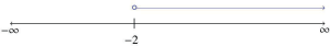
The verbal description is “x is greater than -2.”
We will often have occasion to combine intervals. There are two basic ways to combine intervals: intersection and union.
Definition 5.1
Suppose A and B are two intervals,
- The intersection of A and B,A ∩ B, is the portion of the real number line that the two intervals have in common.
- The union of A and B,A ∪ B, is the portion of the real number line which includes all points of either interval.
Said differently, the intersection of two intervals consists of all real numbers both in the over- lap of the two intervals. The union of two intervals consists of all real numbers in one interval or the other interval or in both. Recall that with events, if A = {1, 2, 3} and B = {2, 4, 6}, then A ∩ B = {2} and A ∪ B = {1, 2, 3, 4, 6}.
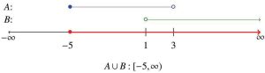
Now, if A is the interval [−5, 3) and B is the interval (1, ∞), both shown in Figure 5.1.5,
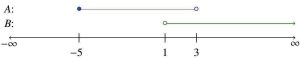
then we can represent A ∩ B graphically. To determine A ∩ B, we shade the overlapping portions of the two line segments and obtain the interval A ∩ B = (1, 3), shown in Figure 5.1.6. Notice the endpoints of the line segment are ‘open’ circles, as the endpoints are not included in both intervals.
We can also represent A ∪ B, graphically by shading all points included in either A or B or both. The resulting shaded region, A ∪ B = [−5, ∞), is shown in Figure 5.1.7. Notice the non-included endpoints of A and B are both included in the union, because they were in at least one of the intervals.
Example 2: Express the following sets of numbers, using interval notation.
(a) {x | x ≤ −2 or x ≥ 2}
(b) {x | x /= 3}
(c) {x | x /= ±3}
(d) {x | x ≤ 4 and x > −2}
Solution: (a) First, let the inequality x ≤ −2 correspond to the interval A : (−∞, −2], and the inequality x ≥ 2 correspond to the interval B : [2, ∞). Then, the best way to proceed is to graph each interval as an equivalent line segment, as shown in Figure 5.1.8.
A : (−∞, −2],B : [2, ∞)
Because of the “or” in the set-builder notation, we are looking to describe the real numbers, x, in A or B, or in both A and B. Considering the intervals have no overlap, we have {x | x ≤ −2 or x ≥ 2} is equivalent to (−∞, −2] ∪ [2, ∞), in interval notation, as shown on the real number line in Figure 5.1.9.
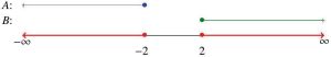
A ∪ B : (−∞, −2] ∪ [2, ∞)
(b) For {x | x /= 3}, we shade the entire real number line except at x = 3, where we leave an ‘open’ circle. (See Figure 5.1.10.)
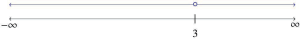
Notice this divides the real number line into two non-overlapping intervals. One being to the left of x = 3, (−∞, 3), and the other being to the right, (3, ∞). As the values of x could only be in one of these intervals, but not both, we have that {x | x /= 3} is equivalent to (−∞, 3) ∪ (3, ∞), in interval notation, as shown in
Figure 5.1.11.
(c) For {x | x /= ±3}, we proceed as in part b and exclude both x = 3 and x = −3
from the real number line, as shown in Figure 5.1.12.
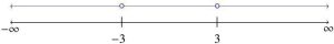
This breaks the real number line into three non-overlapping intervals: (−∞, −3), (−3, 3), and (3, ∞). The set describes real numbers which come from the first, second, or third interval, so we have {x | x /= ±3} is equivalent to (−∞, −3)∪(−3, 3)∪(3, ∞), in interval notation, as shown in Figure 5.1.13.
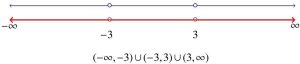
While we say x is not equal to -3 and x is not equal to 3, it is important to note the graphical representation gives three unique intervals which make our statement true. All possible values of x in these unique intervals must be included in our corresponding interval notation. Because the intervals do not intersect, if we used an intersection symbol, ∩, in the interval notation (as the word ’and’ usually indicates), the subsequent interval would be empty. Therefore, we use the union symbol, ∪, to join intervals when writing interval notation.
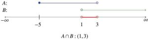
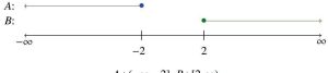
(d) Let the inequality x ≤ 4 correspond to the interval A : (−∞, 4] and the inequality x > −2 correspond to the interval B : (−2, ∞). Now proceed as in part a, by graphing these intervals as equivalent line segments. (See Figure 5.1.14.)
![Two number lines labeled A and B. Line A has a green dot at 4, representing the interval (-∞, 4]. Line B has an open circle at -2 and extends to the right toward infinity, representing the interval (-2, ∞).](https://iu.pressbooks.pub/app/uploads/sites/2011/2025/02/image14-1-300x78.jpeg)
Because of the “and” in the set-builder notation, we are looking to describe the real numbers, x, in the overlapping portions of interval A and interval B. In doing so, we have {x | x ≤ 4 and x > −2} is equivalent to {x | −2 < x ≤ 4} = (−2, 4], in interval notation. (See Figure 5.1.15.)

(−2, 4]
Try It 0

Specify the Graphed set using an equivalent:
(a) Verbal Description
(b) Set-builder notation
(c) Interval notation
Try It 1
Write the given sets, using interval notation.
(a) {x | x = 0 and x = ±6}
(b) {x | x < 3 or x ≥ 2}
(c) {x | −5 ≤ x < 7 and x = 65
5.3 Differentiating Between a Relation and a Function
Recall in Section 2.2, we said “the natural world is full of relationships between quantities that change.” We briefly explored the idea of a linear function to demonstrate relationships between some business quantities. We will now further investigate a broader collection of relationships, called relations, which include functions.
Definition 5.2
A relation is a set of ordered pairs in the coordinate plane.
The set consisting of the first components of each ordered pair is called the inputs, and the set consisting of the second components of each ordered pair is called the outputs.
We can describe a relation verbally, using a list, or using set-builder notation. By definition the elements in a relation are points in the plane, and, therefore, we often try to describe a relation graphically or algebraically, as well. Depending on the situation, one method may be easier or more convenient to use than another.
As an example, consider the relation R = {(−2, 1), (4, 3), (0, −3)}. As written, R is described as a list. Because R consists of points in the plane, we can plot the points. Doing so produces the graph of R in Figure 5.1.17.
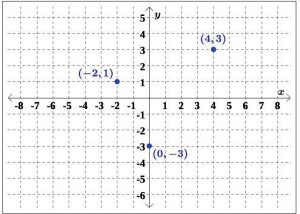
The first number in each ordered pair of the relation makes up the set of inputs, while the second number in each ordered pair makes up the set of outputs. For R, we have
Inputs: {−2, 0, 4} Outputs: {−3, 1, 3}
Note: For sets with a finite number of elements like these, the elements do not have to be listed in particular order. Commonly, they are listed in ascending numerical order, as shown here for R.
One of the core concepts in this text, and in calculus, is the function. There are many ways to describe a function, and we begin by defining a function as a special kind of relation.
Definition 5.3
A relation in which each x-coordinate is matched with only one y-coordinate is said to describe y as a function of x.
In other words a function, f , is a relation that assigns a single element in the set of outputs to each element in the set of inputs, meaning no x-values are repeated. Figures 5.1.18 and 5.1.19, below, show examples of functions, while Figure 5.1.20 shows a relation which is not a function.
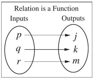
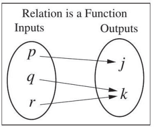
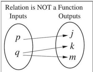
Note: Two different inputs can be associated with one output, but one input cannot be associated with two different outputs.
Note: All functions are relations, but not all relations are functions.
Example 3 The coffee shop menu shown in Figure 5.1.21 consists of items and their prices.
(a) Is the price a function of the item?
(b) Is the item a function of the price?
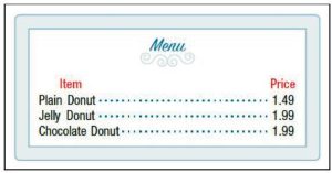
Solution: (a) To determine whether or not the price is a function of the item, consider the input values as the items on the menu, and the output values as the prices. This input/output relation is shown with arrows from the items to the prices in Figure 5.1.22.
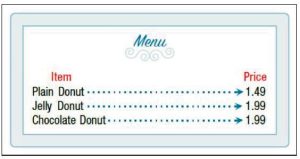
As each item on the menu has only one price, the price IS a function of the item.
(b) To determine whether or not the item is a function of the price, consider the input values as the prices on the menu, and the output values as the items. This input/output relation is shown with arrows from the prices to the items in Figure 5.1.23.
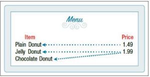
Notice, two items on the menu have the same price. So the same input value has more than one output associated with it. Therefore, the item is NOT a function of price.
In the discussion of functions, we often use the terms domain and range in place of the terms inputs and outputs.
Definition 5.4
For any function,
- Each value in the domain of the function is also known as an input value, or independent variable value, and is often labeled with the lowercase letter x.
- Each value in the range of the function is also known as an output value, or dependent variable value, and is often labeled with the lowercase letter y.
The x and y correspond to their position in an ordered pair.
Example 4: Determine whether or not the following relations describe y as a function of x. If the relation describes a function, give the function’s domain and range.
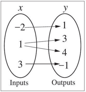
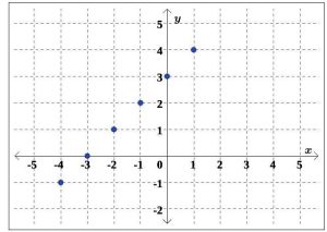
(a) R1 = {(−2, 1), (1, 3), (1, 4), (3, −1)}
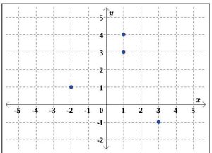
(b) R2 = {(−2, 1), (1, 3), (2, 3), (3, −1)}
Solution: (a) A quick scan of the points in R1 reveals that the x-coordinate 1 is matched with two different y-coordinates: 3 and 4. Hence, in R1,y is not a function of x. To verify, we can draw a picture of the relation. (See Figure 5.1.24.)
(b) Every x-coordinate in R2 occurs only once which means each x-coordinate has only one corresponding y-coordinate. So, R2 does represent y as a function of x. To verify, we can draw a picture of the relation. (See Figure 5.1.25.)
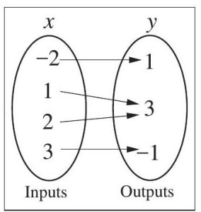
The domain of the function is {−2, 1, 2, 3}. The range of the function is {1, 3, −1}. (Note, as we have a finite number of values, the order in which they are listed does not matter.)
Try It 0
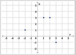
Determine whether or not the relations graphed in Figures 5.1.26 and 5.1.27 represent y as a function of x. If the relation is a function, state the function’s domain and range.
(a)
(b)
Figure 5.1.27: A coordinate plane with points at
(−4, −1),(−3, 0),(−3, 1),(−2, 1),(−1, 2),(0, 3), and (1, 4).
To see what the function concept means geometrically, we graph R1 and R2 from the previous example in the coordinate plane in Figures 5.1.28 and 5.1.29, respectively.
R1 = {(−2, 1), (1, 3), (1, 4), (3, −1)}
R2 = {(−2, 1), (1, 3), (2, 3), (3, −1)}
From the definition of a function, we have already determined that R1 is not a function, by the fact that the x-coordinate 1 is matched with two different y-coordinates in R1. This presents itself graphically as the points (1, 3) and (1, 4) lying on the same vertical line, x = 1.
We have already determined that R2 is a function. In the graph of R2, we see that no two points of the relation lie on the same vertical line. We can generalize these ideas in the following test.
Theorem 1 The Vertical Line Test
A set of points in the plane represents y as a function of x if and only if no two points lie on the same vertical line.
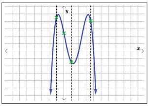
Consider the following graphs in Figures 5.1.30, 5.1.31, and 5.1.32.
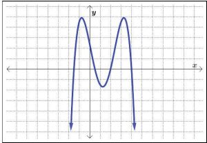
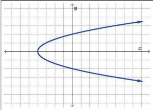
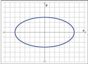
Practically speaking, the Vertical Line Test says that if we can draw any vertical line that intersects a graph more than once, then the graph does not define a function and it fails the Vertical Line Test. Using the Vertical Line Test, we can see in Figures 5.1.33, 5.1.34, and
5.1.35 that only the first of the three graphs represents a function, as the last two graphs fail the Vertical Line Test.
5.1.30 with multiple vertical lines drawn on the graph.
5.1.30 with multiple vertical lines drawn on the graph.
5.1.32 with one vertical line drawn on the graph.
Note: In the graphs of Figures 5.1.34 and 5.1.35 above, we showed only one vertical line passing through the graph of the relation. It is important to mention there are infinitely many vertical lines which could have been drawn, but if a single vertical line intersects the graph more than once, the relation fails the Vertical Line Test, and, thus, the relation is not a function. In general, if all vertical lines intersect the graph in at most one point, the relation passes the Vertical Line Test and is a function, as shown with the multiple vertical lines drawn in Figure 5.1.33.
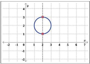
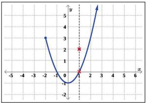
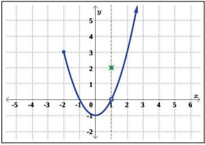
Example 5: Use the Vertical Line Test to determine if any of the following relations, R, S, T , and U , in Figures 5.1.36, 5.1.37, 5.1.38, and 5.1.39, respectively, describe y as a function of x.
(a)
(b)
(c)
(d)
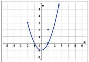
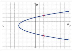
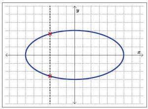
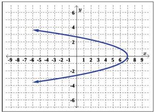
Solution: (a) Looking at the graph of R, we can easily imagine vertical lines intersecting the graph more than once. An example of one such line is graphed in Figure 5.1.40. Hence, R does not represent y as a function of x.
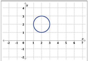
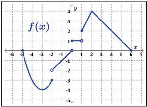
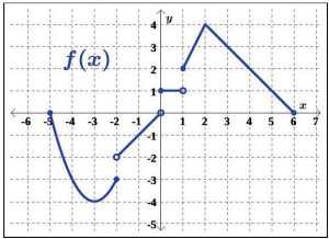
Relations T and U are slight modifications of the relation S, whose graph we determined passed the Vertical Line Test. In both T and U , it is the addition of the point (1, 2) which threatens to cause trouble.
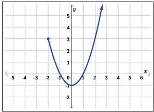
(b) In the graph of T , there is a point on the curve with x-coordinate 1 just below (1, 2), which means that both (1, 2) and this point on the curve, (1, 0), lie on the vertical line x = 1. (See Figure 5.1.42.) Hence, the graph of T fails the Vertical Line Test, so y is not a function of x.
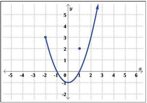
(c) In the graph of U , notice that the point with x-coordinate 1 on the curve has been omitted, leaving an ’open’ circle there. Hence, the vertical line x = 1 intersects the graph of U only at the point (1, 2). Indeed, any vertical line will intersect the graph at most once, so we have that the graph of U passes the Vertical Line Test. (See Figure 5.1.43.) Thus, U represents y as a function of x.
Try It 1
Determine whether or not the given relation graphed in Figure 5.1.44, below, represents y as a function of x.
We now will demonstrate how to determine the domain and range of functions given to us graphically.
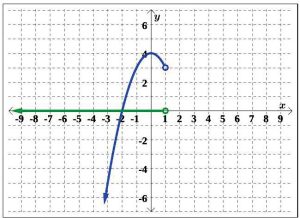
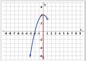
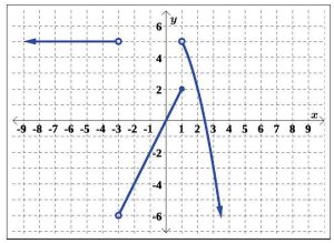
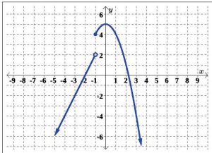
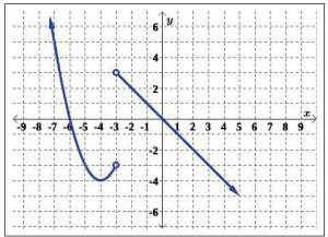
Suppose we are asked to state the domain and range of the function G, whose graph is given in Figure 5.1.45, below.
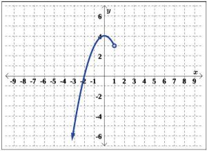
To state the domain and range of G, we need to determine which x – and y-values occur as coordinates of points on the given graph.
To illustrate the domain, it may be helpful to imagine collapsing the curve onto the x-axis and determining the portion of the x-axis that gets covered. This is called projecting the curve to the x-axis (See Figure 5.1.46). Before we start projecting, we need to pay attention to two subtle notations on the graph. The arrowhead on the lower left corner of the graph indicates that the graph continues to curve downwards to the left forevermore, and the open circle at (1, 3) indicates that the point (1, 3) is not on the graph, but all points on the curve leading up to that point are on the graph.
We see from Figure 5.1.47 that if we project the graph of G to the x-axis, we get all real numbers less than 1. Using interval notation, we write the domain of G as (−∞, 1).
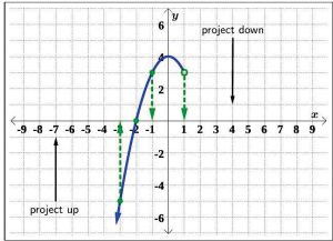
To determine the range of G, we similarly project the curve to the y-axis, as seen in Figure 5.1.48.
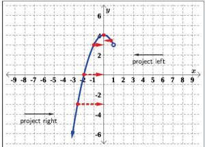
Notice that even through there is an ‘open’ circle at (1, 3), we still included the y-value of 3 in our range, as the point (−1, 3) is on the graph of G. We see that the range of G is all real numbers less than or equal to 4, or, in interval notation, (−∞, 4].
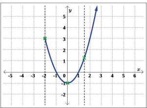
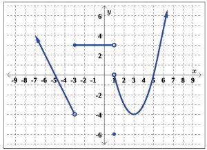
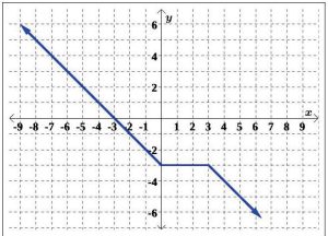
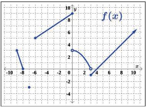
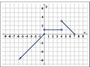
Example 6 State the domain and range of the function given in Figure 5.1.50, using interval notation.
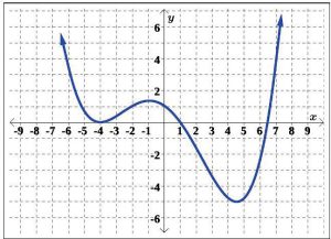
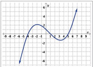
Solution: Before we project the function onto the axes to determine the domain and range, notice the graph extends indefinitely upward to the left and right, as indicated by the arrow heads on the ends of the graph. To illustrate the domain, project the graph up and down to the x-axis, as shown in Figure 5.1.51.
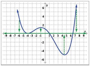
We can see the entire x-axis is included in Figure 5.1.51, if we project the graph to the x-axis. Therefore, the domain includes all real numbers. Using interval notation, we write the domain as (−∞, ∞). To illustrate the range, project the graph left and right to the y-axis, as shown in Figure 5.1.52.
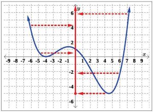
We can see all real numbers greater than or equal to -5 are included in Figure 5.1.52, if we project the graph to the y-axis. Thus, the range includes all real numbers greater than or equal to -5. Using interval notation, we write the range as [−5, ∞).
Try It 2
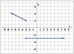
State the domain and range of the function in Figure 5.1.53, below, using interval notation.
5.4 Using Function Notation
Once we determine that a relation is a function, we need to define and display the functional relationship so that we can understand and use it. Sometimes we also need the function in a form so that we can program the function into graphing calculators and computers. There are various ways of representing functions.
Recall from Chapter 2, we used standard function notation when representing the linear busi- ness models. For example, the total cost of producing x items was written as C(x) = mx+F , and the revenue from selling x items was written as R(x) = px.
Remember, we can use any letter to name a function; the notation f (x) shows us that f depends on x. The x-value must be input into the function, f , to obtain a resulting output. The parentheses indicate that x is the input of the function; they do not indicate multiplication.
Definition 5.5
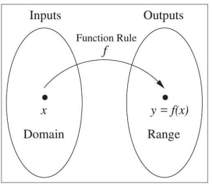
The notation y = f(x) defines a function named f. This is read as “y is a function of x.”
The letter x represents the input value, or independent variable value. The set of all input values is the domain of f. The letter y, or f(x), represents the output value, or dependent variable value. The set of all output values is the range of f.
This relationship is typically visualized using a diagram similar to the one in Figure 5.1.54 below.
Example 7: Use function notation to represent a function whose input is the name of a month and whose output is the number of days in that month.
Solution: The name of the month is the input to a rule that associates the specific number of days in that month (the output) with each input. If we name the rule, or function, f , we write
days = f (month) or d = f (m)
The notation d = f (m) reminds us that the number of days, d (the output), is dependent on the name of the month, m (the input). For example, f ( June ) = 30, because June has 30 days.
30 = f (June)
↑ ↑ ↑
output rule input
Note: The inputs to a function do not have to be numbers; function inputs can be names of people, labels of geometric objects, or any other element that determines some kind of output. However, most of the functions we will work with in this book will have numbers as inputs and outputs.
Example 8: A function N = f (y) gives the number of police officers, N , in a specific town in yearly. What does f (2005) = 300 represent?
Solution: We are given N = f (y), so when we read f (2005) = 300, we see the input, y, is the year 2005. The value for the output, the number of police officers, N , is 300. Thus, the statement f (2005) = 300 tells us that in the year 2005 there were 300 police officers in this specific town.
Try It 1
Use function notation to express the weight of a pig, w (in pounds), as a function of its age in days, d.
When a table represents a function, corresponding domain and range values can also be specified using function notation.
Example 9: Use the function notation g(x) = y to represent the function information given in each row of Table 5.3.
| Domain | Range |
| 2 | 1 |
| 5 | 3 |
| 8 | 6 |
Table 5.3: A table of domain values and corresponding range values for the function g(x).
Solution: The values in the first column are from the domain of the function, and the values from the second column are the corresponding values in the range. Thus, when x = 2,y = g(x) = 1. Using function notation the information can be written as g(2) = 1. Therefore, the corresponding function notation for the information in the remaining rows would be g(5) = 3, when x = 5 and y = g(x) = 3 and g(8) = 6, when x = 8 and y = g(x) = 6.
Try It 2
Use the function notation k(x) = y to represent the function information given in each row of Table 5.4.
Domain Range
1 10
2 100
3 1000
Table 5.4: A table of domain values and corresponding range values for the function k(x).
When a function is defined algebraically and we know an input value, we can determine the corresponding output value of a function by evaluating the function. Evaluating a function will always produce one result (or function value), because each input value of a function corresponds to exactly one output value.
We can also have an algebraic expression as the input value of a function. For example, f (a + b) means “first add a and b, and the result is the input for the function f .” The result when evaluating a function at an algebraic expression is often another algebraic expression in the same variable(s).
Using and evaluating functions are key skills for success in this and many other math courses.
Example 10: Let f (x) = −x2 + 3x + 4. Evaluate and simplify the following.
(a) f (−1),f(0),f(2),f(a)
(b) f (2x), 2f (x)
(c) f (a + b),f(x + 2),f(x)+ 2,f(x)+ f (2)
Solution: (a) To evaluate f (−1), we replace every occurrence of x in the function f (x) with -1. Then, we use order of operations to simplify.
f (−1) = −(−1)2 + 3(−1) + 4
= −(1) + (−3) + 4
= 0
Similarly,
f (0) = −(0)2 + 3(0)+4
= 4
f (2) = −(2)2 + 3(2)+4
= −(4) + 6 + 4
= −4+6+4
= 6
f (a) = −(a)2 + 3(a)+4
= − a2 + 3a +4
= −a2 + 3a +4
(b) To evaluate f (2x), we replace every occurrence of x in the function f (x) with the quantity 2x, and simplify.
f (2x) = −(2x)2 + 3(2x)+4
= − 4x2 + (6x)+4
= −4x2 + 6x +4
The expression 2f (x) means we multiply the function f (x) by 2.
2f (x) = 2 −x2 + 3x +4
= −2x2 + 6x +8
(c) To evaluate f (a + b), we replace every occurrence of x in the function f (x) with the quantity a + b.
f (a + b) = −(a + b)2 + 3(a + b)+4
= −[(a + b)(a + b)] + 3(a + b)+4
= − a2 + 2ab + b2 + (3a + 3b)+4
= −a2 − 2ab − b2 + 3a + 3b +4
To evaluate f (x + 2), we replace every occurrence of x in the function f (x) with the quantity x + 2.
f (x + 2) = −(x + 2)2 + 3(x + 2)+4
= −[(x + 2)(x + 2)] + 3(x + 2)+4
= − x2 + 4x + 4 + (3x + 6)+4
= −x2 − 4x − 4+ 3x +6+4
= −x2 − x +6
To compute f (x)+ 2, we add 2 to the function f (x).
f (x)+2 = −x2 + 3x + 4 +2
= −x2 + 3x +6
From our work in part a, we see f (2) = 6, so
f (x)+ f (2) = −x2 + 3x + 4 +6
= −x2 + 3x + 10
In the previous example, when simplifying −(2x)2, 2x is squared and then multiplied by -1, so that −(2x)2 = −4x2. Also, (a + b)2 = (a + b)(a + b) = a2 + 2ab + b2.
Be careful and watch the order of operations when evaluating functions:
−(2x)2 /= (−2x)2
(a + b)2 /= a2 + b2
Try It 3
Let f(x) = −2×2 − 6x + 5. Evaluate and simply the following.
(a) f(1) (b) f(−x) (c) f(x + h)
Try It Answers
1.
(a) “all real numbers, x, that are less than or equal to -2 or that are between -1 and 3, including -1.”
(b) {x | x ≤ −2 or −1 ≤ x < 3}
(c) (−∞, −2] ∪ [−1, 3)
2.
(a) (−∞, −6) ∪ (−6, 0) ∪ (0, 6) ∪ (6, ∞)
(b) (−∞, ∞)
(c) −5, 6 ∪ 6 , 7
3.
(a) y IS a function of x
Domain: {−4, −3, −2, −1, 0, 1}
Range: {−1, 0, 1, 2, 3, 4}
(b) y is NOT a function of x
4.
y IS a function of x
5.
Domain: (−∞, −3) ∪ (−3, ∞)
Range: (−∞, 5]
6.
w = f (d), where d = age (in days) and w = weight (in pounds).
7.
k(1) = 10, k(2) = 100, k(3) = 1000
8.
(a) f (1) = −3
(b) f (−x) = −2x2 + 6x +5
(c) f (x + h) = −2x2 − 4xh − 2h2 − 6x − 6h +5
Exercises
Basic Skills Practice
For Exercises 1 – 3, express each of the following using equivalent interval notation.
1.
![]()
2.
3.
For Exercises 4 – 7, express each of the following using equivalent interval notation.
4. {x | x ≤ −3} 6. {x | x > 6}
5. {x | x ≥ 20} 7. {x | x < − 5/9 }
For Exercises 8 – 11, determine if the graph of the relation is a function.
8.
9.
10.
11.
For Exercises 12 – 15, use the given graph of f (x) to compute each function value.
12. f (0) 14. f (−3)
13. f (2) 15. f (1/2)
For Exercises 16 – 19, use the given graph of f (x) to determine all values of x where the given function value occurs.
16. f (x) = 0 18. f (x) = −3
17. f (x) = 2 19. f (x) = 1/2
For Exercises 20−22, use the function notation h(x) = y to represent the function information given in each row of the tables below.
20.
21.
| Domain | Range |
| -1 | -2 |
| -2 | -1 |
| 9 | 0 |
Intermediate Skills Practice
For Exercises 23 – 26, express each of the following using equivalent interval notation.
23.
![]()
24.
![]()
25.
![]()
26.
For Exercises 27 – 30, express each of the following using equivalent interval notation.
27. {x | x ≥ −3.4 and x < 100}
28. {x | x > −5 and x ≤ 9, but x /= 0 and x /= 3}
29. {x | x < −1 or x > 7}
30. {x | x < 10 or x > 20, but x /= 30}
For Exercises 31 – 33, state the inputs and outputs of each relation. Then, determine if the relation is a function.
31. {(1, 1), (2, 2), (3, 4)}
32. {(−1, −2), (0, 1), (1, −3), (2, 1)}
33. {(−2, −5), (1, 3), (2, 0), (1, 4)}
For Exercises 34 – 39, use the given graph of f (x) to compute each function value.
34. f (0) 37. f (7)
35. f (4) 38. f (5)
36. f (−3) 39. f − 3/2
For Exercises 40 – 45, use the given graph of f (x) to determine all values of x where the given function value occurs.

40. f (x) = 0 43. f (x) = −1
41. f (x) = 3 44. f (x) = 5
42. f (x) = −3 45. f (x) = 9
For Exercises 46 – 54, use the function f (x) = 2x +1 to evaluate and simplify each of the following.
46. f (3)
47. f (4a)
48. f (a − 5)
49. f (−3)
50. 4f (a)
51. f (a) − f (5)
52.
|
f 3
53.
|
f (a)
54. f (a) − 5
For Exercises 55 – 63, use the function f (x) = 2x2 − x − 12 to evaluate and simplify each of the following.
55. f (0)
56. f (−a)
57. f (a + 5)
58. f (1)
59. −f (a)
60. f (a)+ f (5)
61.
|
f 1
62.
|
f (a)
63. f (a)+5
Mastery Practice
For Exercises 64 – 66, determine if the graph of the relation is a function. If the graph is a function, state the domain and range.
64.
65.
66.
For Exercises 67-72, use the function f (x) = 2 − 1 x to evaluate and simplify each of the
|
following.
67. f (−12)
68. f (2a)
69. f (x)+ h
70. f 3
71.
|
6f (a)
72. f (x + h)
For Exercises 73 − 78, use the function f (x) = −3x2 + 5x +1 to evaluate and simplify each of the following.
73. f (−4)
74. f (a + b)
75. f (x − h)
76. f (1.6)
77. f (a)+ f (b)
78. f (x + h) − f (x)
Communication Practice
- Write the verbal description for (−∞, −12) ∪ (−12, ∞).
- Write the verbal description for (−∞, −7] ∪ (−1, 4).
- Explain why vertical lines are used to determine if the graph of a relation is a function.
Media Attributions
- image1-2
- image2-2
- image3-2
- image4-2
- image5-2
- image6-2
- image7-2
- image8-1
- image9-1
- image10-1
- image11-1
- image12-1
- image13-1
- image14-1
- image15-1
- image16-1
- image17-1
- image18-1
- image19-1
- image20-1
- image21-1
- image22-1
- image23-1
- image24-1
- image25-1
- image26-1
- image28-1
- image29-1
- image30-1
- image31-1
- image32-1
- image33-1
- image34-1
- image35-1
- image36-1
- image37-1
- image38-1
- image39-1
- image40-1
- image41-1
- image42-1
- image43-1
- image44-1
- image45-1
- image46-1
- image47-1
- image48-1
- image49-1
- image50-1
- image51-1
- image52-1
- image53-1
- image54-2
- image55-2
- image56-2
- image57-2
- image58-2
- image59-2
- image60-2
- image61-2
- image62-2
- image63-2
- image64-2
- image65-2
- image66-2
- image67-2
- image68-2
- image69-2
- image70-2
- image71-2
- image72-2