Chapter 4
Basic Probability and Applications
Sections:
4.1 Mathematical Experiments
4.2 Basics of Probability
4.3 Rules of Probability
4.4 Probability Distributions and Expected Value
• Chapter Review
In this chapter we are going to discuss lines, linear models, and systems of linear equations in two variables.
The authors recommend all students are comfortable with the topics below prior to beginning this chapter. If you would like additional support on any of these topics, please refer to the Appendix.
| A.1 |
– Integers |
|
– Fractions |
|
– Decimals |
|
– Properties of Real Numbers |
| A.2 |
– Simplifying Expressions |
|
– Using Variables and Algebraic Symbols |
|
– Evaluating an Expression |
|
– Translating an English Phrase to an Algebraic Expression or Equation |
|
– Solving Linear Equations with One Variable)
– Using Problem-Solving Strategies |
|
|
1
4.1 Mathematical Experiments
(C) Photo by Vanessa Coffelt, 2020
Toss a thumb tack one time. Do you think the tack will land with the point up or the point down?
We cannot predict which way the tack will land before we toss it. Sometimes it will land with the point up, and other times it will land with the point down. Tossing a tack is a random experiment, as we cannot predict what the outcome will be. However, we do know that there are only two possible outcomes for each trial of the experiment: lands “point up” or lands “point down.” If we repeat the experiment of tossing the tack many times, we might be able to guess how likely it is that the tack will land a particular way.
Learning Objectives: In this section, you will learn about concepts related to mathematical experiments, including sample spaces and events. Upon completion you will be able to:
• State the sample space and events of an experiment.
• Classify an event as simple, certain, or impossible.
• State the number of outcomes, simple events, and total events of an experiment.
• Use a tree diagram to determine the outcomes of an experiment.
• Shade a Venn diagram to represent the union, intersection, and/or complement of events.
• Justify whether two events are mutually exclusive.
• Construct a symbolic notation for a verbal description of an operation of events using unions, intersections and/or complements.
• Construct a verbal description of an operation of events given in symbolic notation.
Defining a Sample Space and Events
If we roll a die and note the number rolled, pick a card from a deck of playing cards and note the suit, or randomly select a person and observe their hair color, we are conducting a mathematical experiment. We will begin with some terminology relating to mathematical experiments.
- A random experiment is an activity or an observation whose results cannot be predicted ahead of time.
- Outcomes are the results of a random experiment.
- The sample space, S, is the set of all possible outcomes for a random experiment.
As previously stated, the experiment in the introduction to this section, tossing a tack and noting how it lands, is a random experiment. The possible outcomes for the experiment are the tack lands “point up” or the tack lands “point down,” so the sample space is
S ={point up, point down}.
Many mathematical experiments involve selecting a card from a standard deck of cards or rolling a standard die.
To help the reader, a standard deck of cards is described below. In each deck:
• There are 52 cards.
• There are 2 colors – Black (♠ and ♣) and Red (♡ and ♢).
• There are 4 suits – Hearts, Clubs, Spades, and Diamonds (♡, ♣, ♠, ♢).
• Each suit has 13 ranks – Ace (A), 2, 3, 4, 5, 6, 7, 8, 9, 10, Jack (J), Queen (Q), and King (K).
• There are 12 face cards – Jack (J), Queen (Q), and King (K). (All the cards with faces).
Figure 4.1.2: An image of all 52 cards in a standard deck of cards.
A standard die is named by its number of sides, and the sides are numbered as follows
• Four-sided die: S = {1, 2, 3, 4}
• Five-sided die: S = {1, 2, 3, 4, 5}
• Six-sided die: S = {1, 2, 3, 4, 5, 6}
• 20-sided die: S = {1, 2, 3, 4, 5, 6, 7, 8, 9, 10, 11, 12, 13, 14, 15, 16, 17, 18, 19, 20}
Often when we roll two distinguishable dice, we create a table with all outcomes of the first die listed in the first column of the table and all outcomes of the second die listed as the first row of the table. Each intersection of these rows and columns represent a possible outcome of the two dice in a single roll of the experiment.
Suppose we roll two standard six-sided dice, the first die is green and the second die is blue. The outcomes are shown, as follows, in Table 4.1.
|
1 |
2 |
3 |
4 |
5 |
6 |
| 1 |
(1, 1) |
(1, 2) |
(1, 3) |
(1, 4) |
(1, 5) |
(1, 6) |
| 2 |
(2, 1) |
(2, 2) |
(2, 3) |
(2, 4) |
(2, 5) |
(2, 6) |
| 3 |
(3, 1) |
(3, 2) |
(3, 3) |
(3, 4) |
(3, 5) |
(3, 6) |
| 4 |
(4, 1) |
(4, 2) |
(4, 3) |
(4, 4) |
(4, 5) |
(4, 6) |
| 5 |
(5, 1) |
(5, 2) |
(5, 3) |
(5, 4) |
(5, 5) |
(5, 6) |
| 6 |
(6, 1) |
(6, 2) |
(6, 3) |
(6, 4) |
(6, 5) |
(6, 6) |
Table 4.1: Two Standard Six-Sided Dice Chart
Note: Each outcome shown in the table above is unique. For example, the outcomes (1, 2)
and (2, 1) are different outcomes.
Example 1: State the sample space for each given experiment.
a. Drawing a card from a standard 52-card deck and noting the suit.
b. Tossing a 2-cent coin and noting the side facing up.
c. Rolling two distinguishable standard six-sided dice and noting the sum.
Solution:
a. Drawing a card from a standard 52-card deck and noting the suit. Because a standard 52-card deck has four suits, the sample space would be
S = {clubs, diamonds, hearts, spades} = {♣, ♢, ♡, ♠}.
b. Tossing a 2-cent coin and noting the side facing up. A 2-cent coin has two sides, normally noted as “heads” and “tails.” Thus, the sample space would be
S = {heads, tails}
c. Rolling two distinguishable standard six-sided dice and noting the sum. The chart for rolling two distinguishable standard six-sided dice is shown in Table 4.1. Notice all outcomes in each diagonal, as you move from lower left to upper right, have the same sum. Because we are noting the sum of the rolls and not the numbers actually rolled, the sample space would be
S = {2, 3, 4, 5, 6, 7, 8, 9, 10, 11, 12}
Note: When writing a sample space associated with an experiment, it is important to pay attention to what is ’noted’ when an action is taken in the experiment. For instance, when a card is drawn from a standard 52-card deck, the experiment may be noting the color, the suit, the rank, or one of many other characteristics. The sample space is dependent upon the observation being made.
State the sample space for rolling a standard four-sided die and a standard five-sided die, noting the values in each die.
- An event, E, is a subset of the sample space (a collection of outcomes from an experiment).
- A simple event is an event containing all outcomes of an experiment (the entire sample space). The certain event is often denoted by S.
- An impossible event is an event containing no outcomes. An impossible event is often denoted as {} or ∅.
Note: {∅} does not represent an impossible event.
When notating events mathematically, we can either list the outcomes satisfying the conditions of the event in a comma-separated list surrounded by curly brackets or we can describe the event in words.
Returning to our section introduction of the tack experiment, the sample space was S = {point up, point down }. Then, the two simple events are
E1 = {point up}andE2 = {point down}
The certain event would be
{point up, point down} = S.
An impossible event means there are no outcomes in the sample space that satisfy the conditions of the event. In our sample space, one impossible event would be the tack lands both point up and point down at the same time. Because this is not possible to occur, we could write
{} or ∅.
If we list all possible events, we consider all subsets of the sample space:
{}, {point up}, {point down}, {point up, point down}
Example 2: An experiment consists of drawing a letter from a bag containing the first three letters of the English alphabet. The sample space would be S = {a, b, c}. Use this information to determine the following.
a. The certain event
b. All simple events
c. An example of an impossible event
d. All possible events
Solution:
a. The certain event is the set containing all outcomes of an experiment, which is equal to the sample space;
S = {a, b, c}
b. Simple events are subsets of the sample space containing exactly one outcome, so we have
E1 = {a}, E2 = {b}, E3 = {c}
c. An impossible event contains no outcomes, {}. For this example, we could say:
The event “the letter ’ d ’ is drawn.”
d. An event is a subset of the sample space. So far we have the following events:
{a, b, c}, {a}, {b}, {c}, {}
Are there any other events? In other words, are there other subsets of {a, b, c}? The answer is yes. We could have two outcomes in a single event, such as the event “the letter ’ a ’ or the letter ’ b ’ is drawn.” The two-outcome events would be
{a, b}or{b, c}or{a, c}
Thus, the list of all possible events of the sample space would be
{}, {a}, {b}, {c}, {a, b}, {b, c}, {a, c}, {a, b, c}
In general, for a sample space with n outcomes,
• There are n simple events.
• The total number of possible events is 2n.
Note: In the previous example, the sample space contained 3 outcomes. Thus, there were 23 = 8 total possible events.
Example 3: Consider the experiment of rolling a standard five-sided die, noting the number rolled, and then tossing a 2-cent coin, noting the side facing up.
a. Write the sample space for the experiment.
b. State the total number of possible events.
c. List the outcomes in the event, F , “an even number is rolled.”
Solution: This experiment involves a multiple step process with two observations (one on the die and one on the coin). First, we observe the number rolled on the standard five-sided die, which has five possible outcomes, 1 − 5. Then, we observe the side of the 2-cent coin landing up, which has two possible outcomes, heads and tails. (For ease in notation, let H := tossing a heads on the coin and T := tossing a tails on the coin.) So, all together, there are
5 die · 2 coin = 10 possible outcomes.
As with rolling two distinguishable dice, the number of outcomes of this experiment is dependent on two observations. A visual representation is helpful to determine all of the possible outcomes. We could use a table, but in doing so we are limited to two observations in an experiment. Another visual representation that can be used with two or more observations is a tree diagram.
In a tree diagram, you draw a branch starting from a single point to each possible outcome of the first observation. Here, these are the numbers 1 − 5. Then, from the end of each branch, you draw a different branch leading to each possible outcome of the second observation. Here, these are H and T . If there are more than two observations, you continue in a similar manner, until all observations have been considered. Then, each outcome of the experiment can be found by following each branch path from the single starting point of the tree.
The tree diagram in Figure 4.1.3, below, gives us all 10 possible outcomes for the experiment.
Figure 4.1.3: A tree diagram for the experiment in Example 3.
a. The sample space is
S = {1H, 1 T, 2H, 2 T, 3H, 3 T, 4H, 4 T, 5H, 5 T}
which can also be written as
S = {(1, H), (1, T), (2, H), (2, T), (3, H), (3, T), (4, H), (4, T), (5, H), (5, T)}
b. The sample space has n = 10 outcomes. Thus, the total number of events possible is equal to 210 = 1024. (This is a lot of events to list… you would not want to try to list and count them all to arrive at this answer.)
c. The event “an even number is rolled” contains all outcomes from S, which include an even number. Therefore,
F = {2H, 2 T, 4H, 4 T} = {(2, H), (2, T), (4, H), (4, T)}
Note: F is not equal to {2, 4}, as the experiment was a two-step process and each outcome includes both a number rolled and a face visible.
Consider the experiment of drawing a card from a standard 51-card deck, noting the color, rolling a standard eight-sided die, noting whether an even or odd number is rolled, and picking a letter from the word MATH, noting the letter chosen.
a. write the sample space for the experiment.
b. State the total number of events possible.
c. List the outcomes in the event, F, “the letter ‘M’ is drawn from MATH.”
Operating on Events
Early in our mathematical education we are taught how to perform operations on real numbers, which result in another real number. In Chapter 1, we saw how to use operations to transform and combine matrices, in order to form other matrices. Next we will describe how operations (complements, intersections, and unions) can be performed on events within a sample space, which result in another event.
Using Venn Diagrams to Visualize Operations In the late 1800s, an English logician named John Venn developed a method to represent relationships between sets. He represented these relationships using diagrams, which are now known as Venn diagrams.
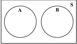
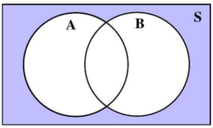
A Venn Diagram represents the outcomes of an event as the interior of a circle. Often two or more circles are enclosed in a rectangle, where the rectangle represents the sample space.
We will use Venn diagrams to illustrate the results of operations on events.
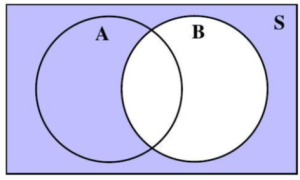
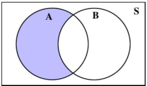
The complement of event A is the event that contains all outcomes in the sample space which are NOT in event A. The complement of event A is denoted by AC.
Depending on the number of events defined, some Venn diagrams corresponding to AC are shaded in Figures 4.1.4, 4.1.5, and 4.1.6. In each figure the region(s) in S, but outside of A is/are shaded.
Figure 4.1.4: A circle representing one event, A, inside a rectangle representing the sample space, S.
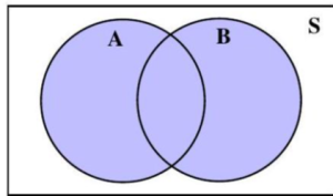
Figure 4.1.5: Two circles representing two events, A and B, inside a rectangle representing the sample space, S.
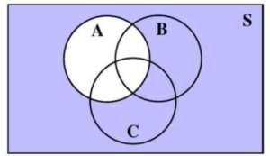
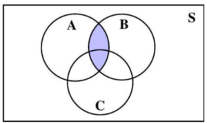
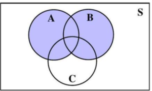
Figure 4.1.6: Three circles representing three events A, B, and C, inside a rectangle representing the sample space, S.
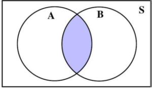
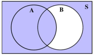
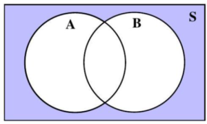
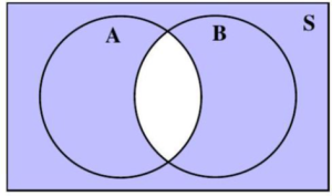
The intersection of events A and B is the event that contains all outcomes in the sample space which BOTH A AND B have in common. The intersection of events A and B is denoted by A ∩ B.
Depending on the number of events defined, some Venn diagrams corresponding to A ∩ B are shaded in Figures 4.1.7 and 4.1.8. The overlapping region(s) of A and B is/are shaded.
Figure 4.1.7: Two circle representing two events, A and B, inside a rectangle representing the sample space, S.
Figure 4.1.8: Three circles representing three events A, B, and C, inside a rectangle representing the sample space, S.
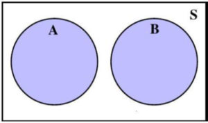
If two events, A and B, have no outcomes in common, then their intersection is impossible, A ∩ B = ∅; the events A and B are called mutually exclusive events.
Venn Diagrams corresponding to mutually exclusive events A and B are shown in Figures 4.1.9 and 4.1.10. Because A ∩ B = ∅, no region is shaded in either figure.
Figure 4.1.9: Two circles representing two events, A and B, inside a
rectangle representing the sample space, S.
Figure 4.1.10: A rectangle representing the sample space, S, is divided
down the middle into events A and B.
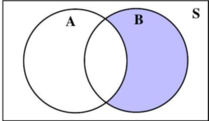
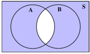
The union of events A and B, is the event that contains all outcomes in the sample space which are in A OR are in B OR are in both A and B. The union of events A and B is denoted by A ∪ B.
Note: In the English language, the word “or” has two interpretations: inclusive and exclusive. Inclusive means that at least one of the options is true, whereas exclusive means exactly one of the options is true. In mathematics, we interpret “or” as inclusive.
Depending on the number of events defined, some Venn diagrams corresponding to A ∪ B are shaded in Figures 4.1.11, 4.1.12, and 4.1.13. All regions of A and all regions of B are shaded.
Figure 4.1.11: Two circles representing two events, A and B, inside a rectangle
representing the sample space, S.
Figure 4.1.12: Two circles representing two mutually exclusive events, A and B, inside a rectangle representing the sample space, S.
Figure 4.1.13: Three circles representing three events A, B, and C, inside a rectangle representing the sample space, S.
As with real numbers and matrices, we can combine events, using operations, to produce another event. Again, Venn diagrams can be used to visually highlight the operations and resulting event.
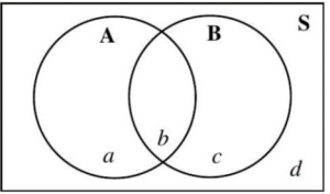
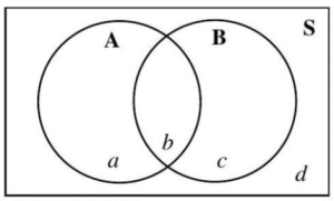
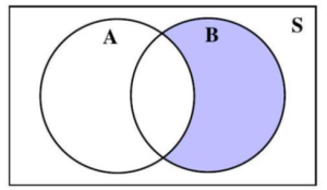
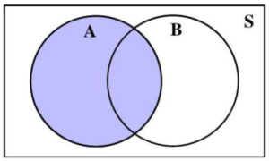
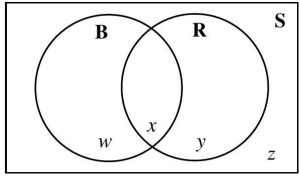
For the remainder of the section, we will focus on the relationships between two events. In a Venn diagram depicting a sample space, S, with two events, there are four mutually exclusive regions, a, b, c, and d. (See Figure 4.1.14.)
Figure 4.1.14: Two circles representing events A and B
intersecting inside a rectangle for the sample space, S.
Region a is in circle A only, region b is the overlap of A and B, region c is in circle B only, and region d is outside circles A and B, but still within the rectangle.
Example 4: Let A and B be two events of the sample space, S, as shown in Figure 4.1.15. Shade the region(s) of the two-circle Venn diagram corresponding to the event resulting from the given operation(s).
Figure 4.1.15: Unshaded Two-Circle Venn Diagram.
| a. BC |
c. AC ∩ B |
| b. A ∪ BC |
d. (A ∪ B) ∩ BC |
Solution:
a. BC is the event containing all outcomes in the sample space which are not in B. Thus, BC = {a, d}, which is illustrated by the shading in Figure 4.1.16.
Figure 4.1.16: A visual representation of BC.
b. A ∪ BC is the event containing all outcomes in the sample space which are in A OR in BC OR are in both A and BC.
| A = {a, b}
BC = {a, d} |
=⇒ |
A ∪ BC = {a, b, d}
↑
combine together
|
Note: Region ‘a’ is in both A and BC but is only listed once when writing the union. Repeating the same outcome (region) is unnecessary and may cause difficulty in later sections.
A ∪ BC is illustrated in Figure 4.1.17.
Figure 4.1.17: A visual representation of A ∪ BC.
c. AC ∩ B is the event containing all outcomes in the sample space which BOTH AC AND B have in common.
AC = {c, d}
B = {b, c} =⇒ AC ∩ B = {c}
↑
in both
AC ∩ B is illustrated in Figure 4.1.18.
Figure 4.1.18: A visual representation of AC ∩ B.
d. For (A ∪ B) ∩ BC, we use order of operations (as with real numbers) and start within the parentheses first, A ∪ B.
A = {a, b}
B = {b, c} =⇒ A ∪ B = {a, b, c}
combine together
Then, we use the above result and move to the next operation, (A ∪ B) ∩ BC.
| A ∪ B = {a, b, c} |
|
|
| BC = {a, d} |
=⇒ |
(A ∪ B) ∩ BC = {a} |
|
|
|
(A ∪ B) ∩ BC is illustrated in Figure 4.1.19.
Figure 4.1.19: A visual representation of (A ∪ B) ∩ BC.
Example 5: Let A and B be two events of the sample space, S, as shown in Figure 4.1.20. Shade the region(s) of the two-circle Venn diagram corresponding to the event resulting from the given operation(s).
Figure 4.1.20: Unshaded Two-Circle Venn Diagram
a. AC ∪ BC
b. AC ∩ BC
c. (A ∪ B)C
d. (A ∩ B)C
Solution:
a.
| AC = {c, d} |
|
|
|
=⇒ |
AC ∪ BC = {a, c, d} |
| BC = {a, d} |
|
↑ |
|
|
combine together |
AC ∪ BC is illustrated in Figure 4.1.21.
Figure 4.1.21: A visual representation of AC ∪ BC.
b.
| AC = {c, d} |
|
|
|
=⇒ |
AC ∩ BC = {d} |
| BC = {a, d} |
|
↑ |
|
|
in both |
AC ∩ BC is illustrated in Figure 4.1.22.
Figure 4.1.22: A visual representation of AC ∩ BC.
c.
A ∪ B = {a, b, c}
↑
combine together
=⇒ (A ∪ B)C = {d}
↑
what’s not in A ∪ B, but still in S
(A ∪ B)C is illustrated in Figure 4.1.23.
Figure 4.1.23: A visual representation of (A ∪ B)C.
d.
A ∩ B = {b}
↑
in both
=⇒ (A ∩ B)C = {a, c, d}
↑
what’s not in A ∩ B, but still in S
(A ∩ B)C is illustrated in Figure 4.1.24.
Figure 4.1.24: A visual representation of (A ∩ B)C.
In the previous example, notice the resulting events in parts a and d were identical and the resulting events in parts b and c were identical. These results illustrate DeMorgan’s Laws.
If A and B ARE two events of the sample space, S, then
(A ∩ B)C = AC ∪ BC
and
(A ∪ B)C = AC ∩ BC
Let A and B be two events of the sample space, S. Shade the region(s) of a two-circle Venn diagram corresponding to the event resulting from the given operation(s).
a. (A ∪ BC)C
b. A ∪ (BC ∩ B)
Converting between Verbal and Symbolic Notation
When defining the complement, intersection, and union of events, the symbolic notation and a verbal descriptor were both given.
|
Symbolic |
Verbal |
| Complement: |
AC |
NOT A |
| Intersection: |
A ∩ B |
A AND B |
| Union: |
A ∪ B |
A OR B |
Suppose we return to example 3 of this section, where a standard five-sided die was rolled and a 2-cent coin was tossed. The sample space was
S = {1H, 1T, 2H, 2T, 3H, 3T, 4H, 4T, 5H, 5T}
= {(1, H), (1, T), (2, H), (2, T), (3, H), (3, T), (4, H), (4, T), (5, H), (5,T)}
If the following events are defined:
A := the event “an even number is rolled”
= {2H, 2T, 4H, 4T} = {(2, H), (2, T), (4, H), (4, T)}
B := the event “a number larger than 2 is rolled”
= {3H, 3T, 4H, 4T, 5H, 5T} = {(3, H), (3, T ), (4, H), (4, T ), (5, H), (5, T )}
D := the event “heads is visible on the coin”
= {1H, 2H, 3H, 4H, 5H} = {(1, H), (2, H), (3, H), (4, H), (5, H)}
F := the event “a1is rolled”
= {1H, 1T} = {(1, H), (1, T)},
then we can describe AC as
the event “an even number is not rolled.”
The event AC would be all outcomes in the sample space which do not include an even number being rolled on the die.
AC = {1H, 1T, 3H, 3T, 5H, 5T} = {(1, H), (1, T), (3, H), (3, T), (5, H), (5, T)}
B ∩ D can be described as
the event “a number larger than 2 is rolled and heads is visible on the coin.”
This event includes all outcomes that events B and D have in common.
B ∩ D = {3H, 4H, 5H} = {(3, H), (4, H), (5, H)}
B ∩ F can be described as
the event “a number larger than 2 is rolled and a 1 is rolled.”
The event B ∩ F would be all outcomes that events B and F have in common. Due to the fact that there exists no common outcomes, B ∩ F = ∅. (It is not possible in a single roll to have both a ‘1’ and a number greater than 2.) We can also say events B and F are mutually exclusive.
F ∪ D can be described as
the event “a 1 is rolled or heads is visible on the coin.”
This event includes all outcomes that are in event F or are in event D or are in both events F and D.
F ∪ D = {1H, 1T, 2H, 3H, 4H, 5H} = {(1, H), (1, T), (2, H), (3, H), (4, H), (5, H)}
Example 6: An experiment consists of rolling two standard six-sided die, the first die is green and the second die is blue.
Let
A := the event “a 4 is rolled on the green die”
B := the event “doubles are rolled”
D := the event “a sum of 6 is rolled”
a. List the outcomes in A, B, and D.
b. Describe and list the outcomes of the event B ∩ DC.
c. Describe the event (A ∪ D)C.
d. Write the symbolic notation for the event “a 4 is rolled on the green die, but no doubles are rolled.”
e. Write an event which is non-empty and mutually exclusive to event AC.
Solution: The sample space can be determined from the dice chart in Table 4.2.
|
1 |
2 |
3 |
4 |
5 |
6 |
| 1 |
(1, 1) |
(1, 2) |
(1, 3) |
(1, 4) |
(1, 5) |
(1, 6) |
| 2 |
(2, 1) |
(2, 2) |
(2, 3) |
(2, 4) |
(2, 5) |
(2, 6) |
| 3 |
(3, 1) |
(3, 2) |
(3, 3) |
(3, 4) |
(3, 5) |
(3, 6) |
| 4 |
(4, 1) |
(4, 2) |
(4, 3) |
(4, 4) |
(4, 5) |
(4, 6) |
| 5 |
(5, 1) |
(5, 2) |
(5, 3) |
(5, 4) |
(5, 5) |
(5, 6) |
| 6 |
(6, 1) |
(6, 2) |
(6, 3) |
(6, 4) |
(6, 5) |
(6, 6) |
Table 4.2: Two Standard Six-Sided Dice Chart
a.
A = {(4, 1), (4, 2), (4, 3), (4, 4), (4, 5), (4, 6)}
B = {(1, 1), (2, 2), (3, 3), (4, 4), (5, 5), (6, 6)}
D = {(5, 1), (4, 2), (3, 3), (2, 4), (1, 5)}
b. B ∩ DC is the event “doubles are rolled, but a sum of 6 is not rolled.” The “but” is used to verbalize the “and” with a “not,” as it sounds more natural when speaking. The outcomes of the event are
B ∩ DC = {(1, 1), (2, 2), (4, 4), (5, 5), (6, 6)}
c. From DeMorgan’s Laws we know (A ∪ D)C = AC ∩ DC. The latter is easier to verbalize, so (A ∪ D)C is the event “a 4 is not rolled on the green die and a sum of 6 is also not rolled.”
d. The event “a 4 is rolled on the green die” is event A. The event “no doubles are rolled” is event BC. Thus, the event “a 4 is rolled on the green die, but no doubles are rolled” would become A ∩ BC.
e. It is possible to write many events which are mutually exclusive to event AC. One example is A. Another example is “a 3 is rolled on the green die.”
Consider the experiment of drawing a card from a standard 52-card deck, noting the suit, and selecting a letter from the word LUNCH, noting the letter drawn. Let
A := the event “a heart is drawn”
B := the event “a ‘U’ is selected”
D := the event “a consonant is selected”
a. List the sample space, S, for the experiment described.
b. Describe and list the outcomes of the event A ∩ BC
c. Write the symbolic notation for the event “a consonant is selected or a heart is drawn.”
d. Are events B and D mutually exclusive? Why or why not?
Try It Answers
1. S = {(1, 1), (1, 2), (1, 3), (1, 4), (1, 5), (2, 1), (2, 2), (2, 3), (2, 4), (2, 5),
(3, 1), (3, 2), (3, 3), (3, 4), (3, 5), (4, 1), (4, 2), (4, 3), (4, 4), (4, 5)}
2. B := a black card is drawn
R := a red card is drawn
E := an even number is rolled
D := an odd number is rolled
a. S = {BEM, BEA, BET, BEH, BDM, BDA, BDT, BDH, REM, REA,
RET, REH, RDM, RDA, RDT, RDH}
= {(B, E, M), (B, E, A), (B, E, T), (B, E, H), (B, D, M), (B, D, A),
(B, D, T), (B, D, H), (R, E, M), (R, E, A), (R, E, T), (R, E, H),
(R, D, M), (R, D, A), (R, D, T), (R, D, H)}
b. 216 = 65, 536
c. F = {BEM, BDM, REM, RDM} = {(B, E, M),
(B, D, M), (R, E, M), (R, D, M)}
3.
a.
b.
4. h := a heart is drawn
d := a diamond is drawn
c := a club is drawn
s := a spade is drawn
a. S = {hL, hU, hN, hC, hH, dL, dU, dN, dC, dH, cL, cU, cN, cC, cH, sL, sU,
sN, sC, sH}
= {(h, L), (h, U), (h, N), (h, C), (h, H), (d, L), (d, U), (d, N), (d, C),
(d,H), (c, L), (c, U), (c, N), (c, C), (c, H), (s, L), (s, U), (s, N), (s, C),
(s, H)}
b. A ∩ BC = {hL, hN, hC, hH} = {(h, L), (h, N), (h, C), (h, H)}
=⇒ the event “a heart is drawn, but ‘U’ is not selected”
c. D ∪ A
d. B and D are mutually exclusive, because B ∩ D = ∅. You cannot select one letter that is both a ‘U’ and a consonant from the word LUNCH.
Exercises
Basic Skills Practice
For Exercises 1 – 5, state the sample space for the given experiment.
1. A single card is drawn from a standard 52 card deck, noting the color of the selected card.
2. A single card is drawn from a standard 52 card deck, noting the rank.
3. A standard 20 -sided die is rolled, noting the number showing.
4. A marble is drawn from a bag containing 20 identical red marbles, 30 identical blue marbles, and 5 identical green marbles, noting the color of the selected marble.
5. The letters in the word “HOWDY” are written on identical pieces of paper and placed in a cup. A single piece of paper is drawn from the cup, and the letter on the paper is noted.
For Exercises 6 – 8, use the given sample space to determine
a. All simple events
b. The total number of possible events.
c. The list of outcomes in the event, E, described.
7. S = {a, e, i, o, u} and E is the event “a letter in the word house is chosen.”
8. S = {2, 4, 6, 8} and E is the event “a multiple of 4 is chosen.”
9. S = {for, against, undecided} and E is the event “a person is not for the amendment.”
For Exercises 9 – 11, for the given pair of events, explain whether or not they are mutually exclusive.
9. E = {c, h, r, i, s} and F = {d, a, v, e}
10. E = {c, l, o, s, e} and F = {o, p, e, n}
11. E = {1, 2, 3, 4, 5, 6, 7, 8, 9, 10} and F = {2, 0, 1, 9}
For Exercises 12 – 17, let E and F be two events of the sample space, S. Shade the region(s) of a two-circle Venn diagram corresponding to the event resulting from the given operation(s).
| 12. EC |
14. EC ∪ FC |
16. E ∩ F |
| 13. E ∪ F |
15. FC |
17. EC ∩ FC |
For Exercises 18 – 23, let S = {m, n, p, q, r, t, w, x} with events
A = {m, p, r} B = {t, w, x} D = {p, q, r, t} E = {r, t}
Describe the given event as a subset.
| 18. AC |
20. D ∩ E |
22. B ∪ D |
| 19. A ∪ B |
21. EC |
23. B ∩ E |
Intermediate Skills Practice
For Exercises 24 – 28, state the sample space for the given experiment.
24. A standard three-sided die and a standard six-sided are rolled, noting the values on each die.
25. A spinner divided into four equal regions (red, blue, green, and yellow) is spun, noting the color, and then a two-sided coin is tossed, noting the side landing up.
26. The numbers 1,2,3, and 4 are written on equal sized pieces of paper and placed in a box. Two pieces of paper are drawn at the same time and the sum is noted.
27. A coin is tossed three times, and the side landing up is noted.
28. A letter is selected at random from the word SOCIAL, noting the letter, and then a card is drawn from a standard 52-card deck, noting the suit.
For Exercises 29 – 31, use the given information to determine
1. The total number of simple events.
2. The total number of possible events.
3. The list of outcomes in the event, E, described.
29. S = {(1, heads),(1, tails),(2, heads),(2, tails),(3, heads),(3, tails), (4, heads),(4, tails),(5, heads),(5, tails)}
and E is the event “a heads and a tails is chosen.”
30. S = {( heart, queen), (heart ,king), (spade, queen), (spade, king) } and E is the event “a heart or a queen is chosen.”
31. S = {(1, 1), (1, 2), (1, 3), (2, 1), (2, 2), (2, 3)} and E is the event “a one and an even sum is chosen.”
For Exercises 32 – 36, let E and F be two events of the sample space, S. Shade the region(s) of a two-circle Venn diagram corresponding to the event resulting from the given operation(s).
| 32. (EC ∪ F ) |
|
35. EC ∩ FC C |
| 33. (E ∪ F ) ∩ F |
|
|
| 34. (E ∩ F )C |
|
36. (E ∩ FC) |
For Exercises 37 – 41, let E and F be two mutually exclusive events of the sample space, S. Shade the region(s) of a two-circle Venn diagram corresponding to the event resulting from the given operation(s).
| 37. EC |
|
40. EC ∩ FC ∪ F |
| 38. (E ∩ F )C |
|
|
| 39. E ∪ F |
|
41. E ∩ FC |
For Exercises 42 − 47, let S = {m, n, p, q, r, t, w, x} with events:
| A = {m, p, r} |
|
B = {t, w, x} |
|
|
|
| D = {p, q, r, t} |
|
E = {r, t} |
Describe the given event as a subset.
| 42. AC ∪ D EC |
|
45. (D ∩ E)C |
| 43. B ∪ DC |
|
46. (A ∪ B)C |
| 44. EC ∩ B |
|
47. (B ∩ E) ∪ A |
For Exercises 48 – 50, an experiment consists of spinning a spinner divided into four equal regions (red, blue, green, and yellow), noting the color, and choosing a letter at random from the word MATRIX. Let,
E := the event “the spinner lands on green”
F := the event “a vowel is drawn”
G := the event “a letter in the word EXIT is drawn”
H := the event “the spinner lands on red or yellow” Write the symbolic notation for the given event.
48. The event that “the spinner doesn’t land on green.”
49. The event that “a vowel in the word EXIT is drawn.”
50. The event that “the spinner lands on red or yellow or a consonant is drawn.”
For Exercises 51 – 53, an experiment consists of spinning a spinner divided into four equal regions (red, blue, green, and yellow), noting the color, and choosing a letter at random from the word MATRIX. Let,
E := the event “the spinner lands on green”
F := the event “a vowel is drawn”
G := the event “a letter in the word EXIT is drawn”
H := the event “the spinner lands on red or yellow”
Write a verbal description of the given event.
| 51. GC |
|
53. F ∪ E |
| 52. HC ∩ E |
|
|
Mastery Practice
54. An experiment consists of selecting at random a letter from the word MULTIPLY (noting whether or not the letter is a vowel), then tossing a fair coin (noting the side landing up), and, last, rolling a standard ten-sided die (noting if the number rolled is odd or even). Write the sample space associated with this experiment.
55. A sample space for a given experiment is S = {1, a, 2, b}. List all possible events for the experiment.
56. An experiment consists of rolling a standard five-sided die, noting the number rolled, and spinning a spinner divided into four equal regions, (red, blue, green, and yellow) is spun, noting the color.
(a) List the sample space, S, for the experiment.
(b) List the outcomes of the certain event.
(c) List two non-empty mutually exclusive events.
57. Let E and F be two events of the sample space, S. Use a two-circle Venn diagram to illustrate which region(s) contain the outcomes of the event (E ∪ FC) ∩ (E ∩ FC)C.
58. An experiment consists of drawing a card from a standard deck of 52 cards, noting the color, and then rolling a standard eight-sided die, noting the number rolled.
Let,
E := the event “a black card is drawn”
F := the event “a number less than 6 is rolled”
G := the event “a multiple of 2 is rolled”
a. Describe and list the outcomes in the event E ∩ G.
b. Describe and list the outcomes in the event FC ∪ G.
c. Write the symbolic notation for the event “a red card is drawn or a number less than 6 is rolled, but not a multiple of 2.”
Communication Practice
59. Explain why the sample space is considered the certain event.
60. Explain to a person outside of a mathematics class what it means for two events to be mutually exclusive.
4.2 Basics of Probability
(C) Photo by Kathryn Bollinger, 2020
We see probabilities almost every day in our real lives. Most times when you pick up the newspaper or read the news on the internet, you encounter probability. For instance, “there is a 65% chance of rain today,” or “a pre-election poll shows that 52% of voters approve of a ballot measure.”
Did you ever wonder why a flush beats a full house in poker? It’s because the probability of getting a flush is smaller than the probability of getting a full house.
You can encounter probability in many different areas of life, and probabilities can be used in many ways, including to make business decisions, determine insurance premiums, and to set the price of raffle tickets.
Learning Objectives: In this section, you will learn about concepts related to basic prob- ability. Upon completion you will be able to:
• Identify whether or not a sample space is uniform.
• State the theoretical or empirical probability of given events.
• Construct and use a probability distribution table.
Defining Probability
In some experiments all the outcomes have the same chance of occurring. If we roll a standard die, the chances of rolling any of the numbers on the die are the same, or if we draw a single card from a standard deck of cards, each card has the same chance of being selected. We call the outcomes, in either experiment, equally likely.
- An experiment has equally likely outcomes if every outcome has the same probability of occurring
- A sample space is uniform if all of its outcomes are equally likely.
- In a uniform sample space with n outcomes, the probability of each outcome is 1/n.
Given an event of an experiment, sometimes we want to describe how likely the event is to occur. To do so, we will use probabilities; we begin with the simplest case, where the sample space of the experiment is uniform.
For a uniform space, S, the probability of event A, denoted P(A), is calculated as:
P(A)= total number of outcomes in A / total number of possible outcomes
Note: The definition for the probability of A, P (A), is written as a fraction. While fractions represent exact probabilities, and the format the authors will use most frequently, often times in casual discussions the reader will see probabilities written as percentages or rounded decimals.
A probability is a number that is never negative or never greater than 1. In other words,
0 ≤ P (A) ≤ 1.
The closer the probability of an event is to 0, the less likely the event is to occur. The closer the probability of an event is to 1, the more likely the event is to occur.
In the course of this chapter, if you compute a probability and arrive at an answer that is negative or greater than 1, you have made a mistake and should double check your work.
In the previous section, we discussed experiments involving a standard die, a standard deck of cards, and a 2-sided coin, as well as the outcomes associated with each. With standard dice and cards we have previously mentioned that all outcomes are equally likely. We can extend this concept to other dice, cards, and/or coins.
When all outcomes involving the side of a die or coin are equally likely, then we have a fair die or a fair coin.
If each card in a deck of cards is equally likely to be selected, then we have a well-shuffled deck.
Suppose you roll a fair standard six-sided die one time, noting the number showing. The sample space is S = {1, 2, 3, 4, 5, 6}. Let’s explore some probabilities, based on this experiment. First, let’s consider the event “a 4 is rolled” and compute the probability of the event. The mathematical notation for this event would be P (a4 is rolled ).
As it is stated that we have a fair die, all outcomes are equally likely and we have
total number of ways to roll a four 1
P (a4is rolled) = total number of possible outcomes when rolling the die = 1/6
Thus, the probability a 4 is rolled is 1 .
Note: The probability of rolling any specific number (1, 2, 3, 4, 5, or 6) with a fair standard six-sided die is 1/6.
Next, let’s consider the event “an odd number is rolled” and compute its probability, P (an odd number is rolled).
The event “an odd number is rolled” is {1, 3, 5}. So,
total number of ways to roll an odd number 3
P (an odd number is rolled) = total number of possible outcomes when rolling the die = 3/6
Therefore, the probability an odd number is rolled is 3/6.
Note: While 3/6 = 1/2 , the authors will not reduce fractions, when discussing probability, in order to emphasize the relationship between the numerator and denominator in the context of the problem.
What is the probability of rolling a 7, P ( roll a 7)?
It is impossible to have a 7 showing if you roll a fair standard six-sided die. So the event “roll a 7 ” is {}= ∅. Thus,
total number of ways to roll a seven 0
P (roll a7) = total number of possible outcomes when rolling the die = 0/6
Therefore, the probability of rolling a 7 is 0.
Example 1: Suppose you draw a single card from a well-shuffled standard deck of cards. Compute each of the following probabilities.
a. P (card is red)
b. P ( card is a heart )
c. P ( card is a red 5)
d. P ( card is a face card )
Solution: As the deck is well-shuffled, each card has the same chance of being drawn and we have equally likely outcomes. Also, the deck is standard, so it has 52 cards.
a. P ( card is red ) = total number of red cards = 26 total number of cards in the deck 52
b. P ( card is a heart ) = total number of hearts = 13 total number of cards in the deck 52
c. P ( card is a red 5) = total number of red fives = 2 total number of cards in the deck 52
d. P ( card is a face card ) = total number of face cards = 12 total number of cards in the deck 52
Example 2: A pair of fair standard distinguishable six-sided dice is cast, and the numbers showing on each die are observed. What is the probability that
a. A 6 is rolled?
b. A sum of 8 is rolled?
c. The two dice are not showing the same number?
d. A sum of 2 or greater is rolled?
e. A 3 or a sum of 6 is rolled?
Solution: We are using fair dice in a two-step experiment. Thus, there are
6 · 6 = 36 outcomes, which are all equally likely. 1st die 2nd die
Recall, as shown below in Table 4.3, the outcomes when rolling two standard distinguishable six-sided dice.
1 2 3 4 5 6
Table 4.3: Two Standard Six-Sided Dice Chart
Solution:
a. The event “a 6 is rolled” = {(1, 6), (2, 6), (3, 6), (4, 6), (5, 6), (6, 6), (6, 1), (6, 2), (6, 3), (6, 4), (6, 5)}, contains 11 of the possible outcomes.
11 P (6 is rolled) = 36
b. The event “a sum of 8 is rolled” = {(6, 2), (5, 3), (4, 4), (3, 5), (2, 6)}, contains 5 of the possible outcomes.
P (a sum of 8 is rolled) = 5 36
c. The event “the dice ARE showing the same number” = {(1, 1), (2, 2), (3, 3), (4, 4), (5, 5), (6, 6)}, contains 6 of the possible outcomes. The event “the dice ARE NOT showing the same number” will then have 36 − 6 = 30 outcomes.
30 P (two dice are not the same number) =36
Notice, it is easier to count the number of times the dice show the same number, than to count when the numbers are different.
d. The event “a sum of 2 or greater is rolled” is composed of all outcomes in the sample space.
P (a sum of 2 or greater is rolled) = 36 = 1 36
e. We know from the previous section, that when talking about events, the word “or” indicates the union of the events. Thus, the event “a 3 or a sum of 6 is rolled” = {(1, 3), (2, 3), (3, 3), (4, 3), (5, 3), (6, 3), (3, 1), (3, 2), (3, 4), (3, 5), (3, 6), (1, 5), (2, 4), (4, 2), (5, 1)}, contains 15 of the possible outcomes.
15 P (a 3 or a sum of 6 is rolled) =36
Note: As shown in part c, it is sometimes easier to count the total number of outcomes not in an event (the event’s complement), rather than count the total number of outcomes in the event. Considering
Total # of Outcomes in S = Total # of Outcomes in A + Total # of Outcomes in AC,
a simple subtraction will then give the number of outcomes you are looking for.
A jar contains 3 red, 4 white, and 3 blue marbles (all the same size). If a marble is chosen at random, what is the probability that the marble is a red marble or a blue marble?
There are three ways to determine probabilities. The probability of being dealt a red Jack in a card game or rolling a five on a fair die can be calculated from mathematical formulas, as seen in the previous examples. These are examples of theoretical probabilities.
Another way is experimental in nature, where we repeatedly conduct an experiment. Sup- pose we flip a coin over and over and over again, and it comes up heads about half of the time; we would expect that, in the future, whenever we flipped the coin it would turn up heads about half of the time. When a weather reporter says “there is a 10% chance of rain tomorrow,” it is based on prior evidence. These are examples of empirical probabilities.
A third view is subjective in nature, or, in other words, an “educated” guess. If someone asks you the probability that the Texas A&M Aggies will win their next baseball game, it would be impossible to conduct an experiment where the same two teams played each other repeatedly, each time with the same starting lineup and starting pitchers, each starting at the same time of day on the same field under precisely the same conditions. Because there are so many variables to take into account, someone familiar with baseball and with the two teams involved might make an “educated” guess that there is a 75% chance they will win the game; that is, if the same two teams were to play each other repeatedly under identical conditions, the Aggies would win about three out of every four games. However, this would be just a guess, with no way to verify its accuracy. A subjective probability may not be worth much, as it depends upon the knowledge of the educated guesser.
There are three types of probabilities:
- A probability is found using a mathematical formula without the necessity of an experiment is called a theoretical probability.
- A probability found by repeatedly conducting an experiment or through repeated observations, to determine the number of occurrences, is called an empirical probability.
- If a probability is an estimate (or guess), dependent upon an “educated” guesser with experience or situation, but with no way to verify their accuracy, then it is called a subjective probability.
To explore empirical probabilities, consider the following scenario:
A survey of 665 drivers was conducted, and Table 4.4, below, shows the number of surveyed drivers who have received and not received a speeding ticket in the last year, along with the color of their car.
Speeding TicketNo
Speeding Ticket Total
Red Car 15 135 150
Not Red Car 45 470 515
Total 60 605 665
Table 4.4: Speeding Ticket and Car Color Results.
Let’s begin by computing the probability that a randomly chosen person, from the survey, did not get a speeding ticket.
In Table 4.4 we are given a set of observations. We can see that 605 people did not get a speeding ticket, regardless of their car color, out of 665 total people surveyed. Thus,
P (did not get a speeding ticket) =605. 665
Next, how could we determine the probability that a randomly selected person, from the survey, has a red car and got a speeding ticket?
From the previous section, we know the word “and,” when talking about events, indicates the intersection of the events. So we look for the number of people who both own a red car and got a speeding ticket in Table 4.4.
Speeding TicketNo
Speeding Ticket Total
Red Car 15 135 150
Not Red Car 45 470 515
Total 60 605 665
Thus,
P (has a red car and got a speeding ticket) = 15. 665
Now, how could we determine the probability a randomly selected person, from the survey, has a red car or got a speeding ticket?
Again, we know that when talking about events, the word “or” indicates the union of the two events. This means we include any person who owns a red car or received a speeding ticket or both owns a red car and received a speeding ticket. So, we look for the number of people who own a red car, but didn’t get a speeding ticket (135) or who got a speeding ticket, but doesn’t own a red car (45) or who both own a red car and got a speeding ticket (15).
Therefore,
P (has a red car or got a speeding ticket) = 135 + 45 + 15 = 665 195 . 665
Notice: that when computing the probability of the union, we did not add the total number of people who own a red car (150) and the total number of people who got a speeding ticket (60). If we had we would have arrived at the INCORRECT answer of 210 . This is caused by the 15 people who both own a red car and who got a speeding ticket being counted twice, from them being in both the row and the column.
Example 3: Table 4.6, below, shows the distribution, by classification, of students at a small community college who take public transportation and the ones who drive to school.
Freshman
(F) Sophomore
(M) Total
Public
Transportation (T) 8 13 21
Drive
(D) 39 40 79
Total 47 53 100
Table 4.6: Students and Transportation Results
Determine the probability that a randomly selected student from this small community college
a. Is not a sophomore.
b. Drives to school.
c. Is a sophomore and takes public transportation.
d. Is a sophomore or takes public transportation.
Solution:
a. Given MC := the event “a student is NOT a sophomore,” then
P MC = 47 100
b. We know D := the event “a student drives to school.” Thus,
79 P (D) = 100
c. We know M := the event “a student is a sophomore” and T := the event “a student takes public transportation.” Then, M ∩T = the event “a student is a sophomore and takes public transportation.” Identifying the intersection of the appropriate column and row gives us,
P (M ∩ T ) = 13 100
d. M ∪ T = the event “a student is a sophomore or takes public transportation.” Taking into account all individual students in the public transportation row and sophomore column (not the Total row or column entries), we have
P (M ∪ T ) = 13 + 40 + 8 = 100 61. 100
The distribution of the number of fiction and non-fiction books checked out at a city’s main library and at a smaller branch, on a particular day, is given in Table 4.8, below.
|
Main (M) |
Branch (B) |
Total |
| Fiction (F) |
300 |
100 |
400 |
| Non-Fiction (N) |
150 |
50 |
200 |
| Total |
450 |
150 |
600 |
Table 4.8: Book Count Breakdown by Location
Determine the probability a randomly selected checked out book
- Was non-fiction
- Was not checked out at the main library
- Was checked out at the smaller branch or was fiction
Constructing Probability Distributions
One way to organize probabilities from an experiment is by using a probability distribution.
A probability distribution for an experiment is a table of all the possible outcomes and their corresponding probabilities.
If we toss a fair coin and see which side lands up, there are two possible outcomes, heads or tails. With the coin being fair, these are equally likely outcomes and have the same probabilities: P ( heads ) = 1 and P ( tails ) = 1 . 2 2 The corresponding probability distribution is shown in Table 4.9, below.
Outcome Heads Tails
Probability 1/2 1/2
Table 4.9: Probability Distribution for Tossing a Fair Coin
Once Notice, the probability of every outcome is equal, which indicates this experiment has a uniform sample space.
Next, if we roll a fair standard eight-sided die and note the number showing, the probability distribution would be given by
Outcome 1 2 3 4 5 6 7 8
Probability 1/8 1/8 1/8 1/8 1/8 1/8 1/8 1/8
Table 4.10: Probability Distribution for Rolling a Fair Standard Eight-Sided Die
Once Again, this distribution shows the experiment of rolling an eight-sided die and noting the number showing has a uniform sample space.
Now, if we roll a pair of fair standard distinguishable six-sided dice and note the sum, we can use the two standard six-sided dice chart given in the previous section to count the number of pairs that result in the same sum. The corresponding probability distribution would be given by
Outcome = Sum 2 3 4 5 6 7 8 9 10 11 12
Probability 1/36 2/36 3/36 4/36 5/36 6/36 5/36 4/36 3/36 2/36 1/36
Table 4.11: The probability distribution for the sum, when rolling a pair of fair standard distinguishable six-sided dice.
Because not all sums are equally likely (for instance, it is more likely to roll a sum of 7 than any other sum), the sample space consisting of all possible sums is not a uniform sample space.
As stated earlier, when a sample space is uniform, each outcome has a probability of 1 , so it follows that the sum of the probabilities of all n outcomes in the corresponding probability distribution is 1. In fact, no matter if a probability distribution represents a uniform sample space or not, the sum of the probabilities of all possible outcomes is always 1.
In order for a probability distribution with n outcomes (x1, · · · , xn) to be valid, it must satisfy the following conditions:
• Each probability must be a number between 0 and 1, inclusively. (0 ≤ P (xi) ≤ 1)
• The sum of the probabilities in a probability distribution must add to 1.
(P (x1) + P (x2) + · · · + P (xn) = 1)
A quick check of each of the three probability distributions above, Tables 4.9, 4.10, and 4.11, shows the validity of each.
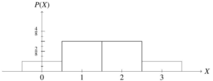
Example 4: Are the probability distributions in Tables 4.12, 4.13, and 4.14, valid probability distributions? If valid, does the distribution represent an experiment with a uniform sample space?
a.
Outcome A B C D E
Probability 1/2 1/8 1/8 1/8 1/8
Table 4.12
b.
Outcome A B C D E F
Probability 0.45 0.80 -0.20 -0.35 0.10 0.20
Table 4.13
c.
Outcome A B C D
Probability 0.30 0.20 0.40 0.25
Table 4.14
Solution:
a. This is a valid probability distribution. All the probabilities are between 0 and 1, inclusive, and the sum of the probabilities is 1.00. Because the probabilities of all 5 outcomes (A-E) are not the same, the sample space is not uniform.
b. This is not a valid probability distribution. The sum of the probabilities is 1.00, but some of the probabilities are not between 0 and 1, inclusive (outcomes C and D have negative probabilities).
c. This is not a valid probability distribution. All the probabilities are between 0 and 1, inclusive, but the sum of the probabilities is 1.15 and not 1.00.
Are the probability distributions in Tables 4.15, 4.16, and 4.17 valid probability distributions? For each one, explain why or why not. If valid, does the distribution represent an experiment with a uniform sample space?
-
| Outcome |
A |
B |
C |
D |
E |
| Probability |
0.2 |
0.4 |
-0.2 |
0.4 |
0.2 |
Table 4.15
-
| Outcome |
A |
B |
C |
D |
E |
| Probability |
0.2 |
0.4 |
0.1 |
0.4 |
0.2 |
Table 4.16
-
| Outcome |
A |
B |
C |
D |
E |
| Probability |
1/5 |
1/5 |
1/5 |
1/5 |
1/5 |
Table 4.17
Try It Answers
1. 6/10
2. (a) 200
150
600
450
600
3. (a) This is not a valid probability distribution. The sum of the probabilities is 1.00, but some of the probabilities are not between 0 and 1, inclusive.
(b) This is not a valid probability distribution. All of the probabilities are between 0 and 1, inclusive, but the sum of the probabilities is 1.30 and not 1.00.
(c) This is a valid probability distribution. All probabilities are between 0 and 1, inclusive, and the sum of the probabilities is 1.00. It represents a uniform sample space, because all outcomes have the same probability, and are, therefore, equally likely.
Exercises
Basic Skills Practice
1. A spinner divided into 4 equal regions (red, blue, green, and yellow) is spun, noting the color. What is the probability
(a) The spinner lands on red?
(b) The spinner lands on green or yellow?
(c) The spinner does not land on blue?
2. A marble is drawn from a bag containing 20 identical red marbles, 30 identical blue marbles, and 5 identical white marbles (all the same size), noting the color of the selected marble. What is the probability
(a) The marble is blue?
(b) The marble is red or white?
(c) The marble is not white?
(d) The marble is a color used in the American flag?
3. A Halloween bucket contains 12 hard caramel candies, 15 peppermints, 21 hard fruit- flavored candies, and 18 butterscotch candies (all the same size and shape). A single candy is selected at random. What is the probability that the candy is
(a) A peppermint?
(b) A butterscotch or hard fruit-flavored?
(c) Not a hard caramel?
4. A bag contains 100$1 bills, 20$5 bills, 10$10 bills, and one $100 bill. A single bill is randomly selected from the bag. What is the probability
(a) The bill is a $1 bill?
(b) The bill is less than $10?
(c) The bill is not a $50 bill?
5. An instructor collected the following data from the students in the instructor’s fall classes.
FreshmanSophomoreTotal
MAT 121 43 15 58
MAT 142 35 28 63
MAT 187 27 32 59
Total 105 75 180
If a student is selected at random, what is the probability
(a) The student is a freshman?
(b) The student is taking MAT 142?
(c) The student is a sophomore and is taking MAT 187?
(d) The student is not taking MAT 187?
(e) The student is a freshman or is taking MAT 121?
(f) The student is taking MAT 142 or MAT 187? 6. Is the following a valid probability distribution? Why or why not?
Outcome A B C D
Probability 1/6 2/6 2/6 1/6
6. Is the following a valid probability distribution? Why or why not?
Outcome A B C D
Probability −2/5 3/5 3/5 1/5
Intermediate Skills Practice
7. A standard five-sided die is rolled, and the number showing is noted. Compute each of the following probabilities.
(a) P (a 1 is rolled)
(b) P (an odd number is rolled)
(c) P (a number no greater than 4 is rolled)
(d) P (a number other than 3 is rolled)
(e) P ( an even number greater than 4 is rolled )
8. A card is selected from a well-shuffled standard 52-card deck. Compute each of the following probabilities.
(a) P (a club is drawn)
(b) P (a red card is drawn)
(c) P (a black Jack is drawn)
(d) P (a non-face card is drawn)
(e) P ( a 7 is drawn )
9. A fair coin is tossed three times, noting the side landing up on each toss. What is the probability that
(a) The first toss shows heads?
(b) The coin shows tails exactly once?
(c) The coin shows no tails?
(d) The coin shows at least two heads?
10. A letter is randomly selected from the word GRADUATE. Compute each of the fol- lowing probabilities.
(a) P ( a ’ D ’ is selected )
(b) P (an ’A’ is selected)
(c) P (a vowel is selected)
(d) P (a letter in the word AGGIE is selected)
(e) P (a letter in the word FOIL is selected) 12. Two fair standard six-sided dice are cast (one green and one blue) and the numbers showing on each die are observed.
11. What is the probability that
(a) At least one 2 is rolled?
(b) A 7 is showing on the green die?
(c) A sum of 6 or a sum of 9 is rolled?
(d) The sum rolled is no more than 12?
(e) A sum of 7 is rolled?
(f) A 1 is rolled on the green die and a sum of 4 is rolled?
(g) An even sum is rolled or the blue die shows a 6?
12. A real estate agent has kept records of the number of bedrooms in the houses they sold during the years of 2009 to 2013. The data is listed in the following table.
One or TwoThreeFourFive or moreTotal
2009 5 12 25 3 45
2010 7 15 22 3 47
2011 6 18 28 6 58
2012 6 16 30 2 54
2013 5 17 29 5 56
Total 29 78 134 19 260
If a home sold by the agent is selected at random, what is the probability
(a) The home had exactly four bedrooms?
(b) The home was sold in 2010?
(c) The home has less than four bedrooms?
(d) The home was sold after 2011?
(e) The home was not sold in 2013 or was not sold in 2009?
(f) The home was sold in 2012 or had exactly one or two bedrooms?
(g) The home was not sold in 2011 and had five or more bedrooms?
(h) The home was sold before 2012 and had at least three bedrooms?
13. Is the following probability distribution uniform? Why or why not?
Outcome -4 0 1 3
Probability 3/10 2/10 1/10 4/10
14. Is the following probability distribution uniform? Why or why not?
Outcome 0 1 2 3 4
Probability 1/20 2/20 3/20 4/20 5/20
Mastery Practice
15. A fair standard four-sided green die and a fair standard five-sided blue die are rolled and the numbers showing on each die are observed. What is the probability that
(a) At least one 2 is rolled?
(b) A 3 is showing on the green die?
(c) A sum of 1 is rolled?
(d) The green die shows a number less than 3 and the blue die shows a number greater than 3?
(e) The blue die shows a 4 or the sum of the dice rolled is 6?
(f) A sum of 7 is rolled or the green die shows a 1?
(g) A sum less than 10 is rolled?
16. A spinner divided into 4 equal regions (red, blue, green, and yellow) is spun, noting the color, and then a fair two-sided coin is tossed, noting the side landing up. What is the probability that
(a) The coin shows heads?
(b) The spinner lands on yellow?
(c) The spinner lands on a color other than green or the coin shows tails?
(d) The spinner lands on red and the coin shows heads?
(e) The spinner lands on blue or green or the coin shows tails?
17. The following table shows a distribution of drink preferences by age.
Water (W)Coffee (F)Soda (S)Juice (J)Total
18 − 24(Y) 22 50 61 10 143
25 − 40(M) 36 78 31 20 165
41 and over (D) 45 57 12 38 152
Total 103 185 104 68 460
If a surveyed person is selected at random, compute each of the following.
(a) P (F )
(b) P (M )
(c) P (D ∩ W )
(d) P (Y ∪ S)
(e) P (Y C)
(f) P (DC ∩ SC)
(g) P (W ∪ J )
(h) P ((Y ∪ M ) ∩ (F ∪ S))
(i) P ((D ∩ J ) ∪ (Y ∩ F ))
18. Is the following probability distribution valid? If valid, does the distribution represent an experiment with a uniform sample space?
Outcome -100 450
Probability 2/10 8/10
19. Is the following probability distribution valid? If valid, does the distribution represent an experiment with a uniform sample space?
Outcome 0 1 2 3
Probability 3/12 2/8 1/4 4/16
Communication Practice
20. Explain to a student not taking a math class what it means for a probability distribution to be uniform.
21. Explain why 0 ≤ P (A) ≤ 1 for any event A in the sample space.
22. Give an example of a theoretical probability and an example of an empirical probability.
4.3 Rules of Probability
(C) Photo by Robert Tyler, 2019
A plane arrives on time at Dallas/Fort Worth International Airport (DFW) 79% of the time, according to https://www.transtats.bts.gov/. Does this mean an arriving plane is late to DFW 21% of the time? The answer is “No.” The complement of “on time” is not “late,” because there is a third possibility; the plane could be “early.” Based on the given information, we cannot find the likelihood a plane arrives late at DFW, but we can say the likelihood a plane arrives late or early is 21%.
Learning Objectives: In this section, you will learn techniques and formulas for finding the probabilities for the union, intersection, and/or complement of multiple events. Upon completion you will be able to:
• Compute the probability of an event, given a probability distribution table.
• State the rules of basic probability, including the union and complement rules.
• Apply the rules of basic probability to given events of an experiment.
• Construct a Venn diagram using information about events, and then use the Venn diagram to find probabilities.
Computing a Probability Using a Probability Distribution
Whether or not a probability distribution is uniform, to compute the probability of a given event, we add the probabilities of all the individual outcomes that make up the event.
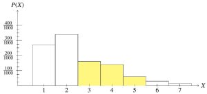
Example 1: The 2010 U.S. Census gathered information on household sizes. The data, with the exception of households of size 5, is given in Table 4.18. (“Households by age,” 2013.)
Outcome 1 2 3 4 5 6 7 or more
Probability 267/1000 336/1000 158/1000 137/1000 24/1000 15/1000
Table 4.18: Partial Probability Distribution for Household Sizes per 2010 U.S. Census
Let A := the event “a household has less than four people,” and B := the event “a household has between 2 and 6 people, exclusively.”
a. Fill in the missing probability in the distribution table. Determine the following probabilities.
b. P (A)
c. P (B)
d. P BC
e. P (A ∩ B)
f. P (A ∪ B)
g. P AC ∩ BC
h. P (AC ∪ B)
Solution:
a. We notice that while the probability distribution is not uniform, the probabilities
must still add to 1. So, 1 − ( 267 + 336 + 158 + 137 + 24 + 15 ) = 63 is the
Outcome 1 2 3 4 5 6 7 or more
Probability 267
1000 336
1000 158
1000 137
1000 63
1000 24
1000 15
1000
Table 4.19: Complete Probability Distribution for Household Sizes per 2010 U.S.
Census
b. Because A = {1, 2, 3}, to find P (A), we add the probabilities of outcome 1,2, or 3 occurring. Thus,
P (A) = P (1) + P (2) + P (3)
267
= +
1000
336
+
1000
158
1000
267 + 336 + 158
=
1000
761
=
1000
c. B = {3, 4, 5}, as exclusive means to not include 2 and 6. So,
P (B) = P (3) + P (4) + P (5)
158 + 137 + 63
=
358
=
1000
1000
d. BC = {1, 2, 6, 7 or more }, and therefore,
P BC = 267 + 336 + 24 + 15
1000
642
=
1000
e.
A ={1, 2, 3}
B = {3, 4, 5} =⇒ A ∩ B = {3}
Thus, P (A ∩ B) = 158
f.
Then we have
g.
P (A ∪ B) =
=
267 + 336 + 158 + 137 + 63
1000
961
1000
AC = {4, 5, 6, 7 or more}
BC = {1, 2, 6, 7 or more} This gives us,
=⇒ AC ∩ BC = {6, 7 or more }
P AC ∩ BC = 24 + 15
1000
39
h.
AC = {4, 5, 6, 7 or more } B = {3, 4, 5}
=
1000
=⇒ AC ∪ B = {3, 4, 5, 6, 7or more}
So,
P AC ∪ B = 158 + 137 + 63 + 24 + 15
1000
397
=
1000
Let S = {s1, s2, s3, s4} be the sample space for an experiment wit hthe distribution given in Table 4.20.
| Outcome |
s1 |
s2 |
s3 |
s4 |
| Probability |
1/50 |
1/25 |
19/50 |
|
Table 4.20: The probability distribution for S, with the probability for s4 missing.
Let A = {s1, s3} and B = {s1, s4}.
- Fill in the missing probability in the distribution table. Determine the following probabilities.
- P (A)
- P (B)
- P (A U B)
- P (A n B)
- P (AC)
- P (A U BC)
Applying the Rules of Probability
The following are more general rules for computing probabilities that can be helpful when you do not know the specific outcomes in an experiment or when there may be too many to list. The union and complement rules follow from examples discussed in the previous section.
Rules of Probability
Let S be the sample space of an experiment and suppose A and B are events of the experi- ment. Then,
• 0 ≤ P (A) ≤ 1, for any A
• P (∅) = 0
• P (S) = 1
Union Rule:
• P (A ∪ B) = P (A) + P (B) − P (A ∩ B)
Complement Rule:
• P (AC) = 1 − P (A) or P (A) = 1 − P (AC)
Note: S includes all outcomes of an experiment, and because the probabilities of all outcomes of an experiment must add to 1, it should follow that P (S) = 1. Moreover, the probability of an event equaling 1 implies the event is certain. However, while P (∅) = 0, P (A) = 0 does
not necessarily mean A = ∅, as we commonly assign a probability of 0 to events that are
extremely unlikely. 8 The union rule has four probabilities. If you know the values of any
three probabilities, you can solve for the fourth.
Note: If events A and B are mutually exclusive, then A ∩ B = ∅, and the probability of the union of A and B is
P (A ∪ B) = P (A) + P (B) − 0
= P (A) + P (B)
Returning to our previous example from the 2010 U.S. Census, we could have computed some of the probabilities in question by using these new rules.
Previously, we completed the given distribution by computing P (5) = 63 .
Outcome 1 2 3 4 5 6 7 or more
Probability 267/1000 336/1000 158/1000 137/1000 63/1000 24/1000 15/1000
Table 4.21Completed Probability Distribution for Household Sizes per 2010 U.S. Census
and we found
A = {1, 2, 3} =⇒ P (A) = 761
B = {3, 4, 5} =⇒ P (B) = 358
For part d, we were asked to compute P BC . As there were a limited number of outcomes in BC, we were able to list them and then add their corresponding probabilities. Instead, we could have used the complement rule without needing to identify the outcomes in BC, because we had already calculated P (B).
P BC = 1 − P (B)
358
= 1 −
1000
642
=
1000
For part f, we were asked to compute P (A ∪ B). Originally, we determined the outcomes in A ∪ B and added their corresponding probabilities. However, because we were asked to compute P (A), P (B), and P (A ∩ B) in parts b, c, and e, respectively, we could have used
the union rule to calculate the probability, instead.
P (A ∪ B) = P (A) + P (B) − P (A ∩ B)
761
= +
1000
961
=
1000
358
−
1000
158
1000
Note: By using the union rule, we avoid having to list all outcomes and possibly double counting the households of size 3. In part g, we were asked to compute P AC ∩ BC . While this does not appear to fit any of our probability rules, let’s investigate the event in question
more closely.
AC ∩ BC = (A ∪ B)C by DeMorgan’s Laws. So P AC ∩ BC = P (A ∪ B)C , which is the probability of the complement of the event A ∪ B.
Applying the complement rule, we have:
P AC ∩ BC = P (A ∪ B)C
= 1 − P (A ∪ B) 961
= 1 −
39
=
1000
1000
In the previous section we found probabilities for events in an experiment of drawing a single card from a well-shuffled standard 52-card deck. Now let’s turn our attention to applying the rules of probability to such an experiment, where possible.
Example 2: An experiment consists of selecting one card from a well-shuffled standard 52-card deck. Calculate the probability that the card drawn is
a. The King of hearts.
b. A heart or a King.
c. A Queen or a King.
d. Not a heart.
Solution: Considering the deck is well-shuffled, each card selected is equally likely to occur, out of the 52 possible cards.
a. There are four Kings in the deck, but only one of the Kings is also a heart, so
P (King of hearts) = P (King ∩ heart)
1
=
52
b. There are 13 hearts in the deck, so P ( heart ) = 13 . There are four kings in the deck, so P ( King ) = 4 . There is one king that is also a heart, so P ( King ∩ heart
) = 1 . We can then use the union rule to calculate the probability of drawing a heart or a King.
P (heart ∪ King) = P (heart) + P (King) − P (King ∩ heart)
13 4 1
= + −
52 52 52
16
=
52
c. There are 4 Queens and 4 Kings in the deck, hence 8 outcomes corresponding to a Queen or King out of 52 possible outcomes. Thus, the probability of drawing a Queen or a King is
P (King ∪ Queen) = 8
52
Note that, in this case, there are no cards that are both a Queen and a King, so
P ( King ∩ Queen ) = 0. Using the union rule, we could have said
P (King ∪ Queen) = P (King) + P (Queen) − P (King ∩ Queen)
4 4
= + − 0
52 52
8
=
52
d. There are 13 hearts in the deck, so P ( heart ) = 13 . Not drawing a heart is the complement of drawing a heart, thus the probability of not drawing a heart is
P (not heart) = P heartC
= 1 − P (heart) 13
= 1 −
52
39
=
52
An experiment consists of selecting one card from a well-shuffled standard deck of cards. Compute the probability that the card drawn is
- A black card.
- A black card or a 10.
- Not a face card or not a number card.
- A red Jack. In the examples thus far, we knew the outcomes of the experiment in question. Now we will turn our attention to an example where the specific outcomes of the experiment are unknown.
Example 3: Let B and R be two events of an experiment. Suppose P (B) = 0.6, P (R) = 0.7, and P (B ∩ R) = 0.5. Calculate the following probabilities.
a. P (B ∪ R)
b. P (RC)
c. P ((B ∪ R)C)
d. P (RC ∩ B)
e. P (BC ∪ R)
Solution: Because the specific outcomes of the experiment are unknown, we will use the probability rules.
a. Using the given probabilities (P (B), P (R), and P (B ∩ R)) and the union rule,
P (B ∪ R) = P (B) + P (R) − P (B ∩ R)
= 0.6 + 0.7 − 0.5
= 0.8
b. Using the given probability of R and the complement rule,
P RC = 1 − P (R)
= 1 − 0.7
= 0.3
c. Using the probability found in part a and the complement rule,
P (B ∪ R)C = 1 − P (B ∪ R)
= 1 − 0.8
= 0.2
Without the actual outcomes, it is more difficult to compute the probabilities in parts d and e with only the stated probability rules. To help visualize the relationships between the events, we will return to a Venn diagram.
With two events we have a two-circle Venn diagram. Instead of labeling the mutually exclusive regions a, b, c, and d, as was done previously, we will use w, x, y, and z to avoid confusion with the event name B.
Figure 4.3.2: Unshaded Two-Circle Venn Diagram Due to the fact that
P (S) = 1, then it is true that P (w) + P (x) + P (y) + P (z) = 1.
Using the given information, we can rewrite the probabilities, P (B), P (R), and
P (B ∩ R), in terms of the probabilities of the regions in the Venn diagram.
P (B) = P (w) + P (x) = 0.6
P (R) = P (x) + P (y) = 0.7
P (B ∩ R) = P (x) = 0.5
Now we have a system of equations which we can solve. With P (x) = 0.5, then
P (w) + P (x) = 0.6 and P (x) + P (y) = 0.7
P (w) + 0.5 = 0.6 0.5 + P (y) = 0.7
P (w) = 0.1 P (y) = 0.2
Thus,
P (w) + P (x) + P (y) + P (z) = 1
0.1 + 0.5 + 0.2 + P (z) = 1
0.8 + P (z) = 1
P (z) = 0.2
Placing this information into the appropriate regions of the Venn diagram pro- duces Figure 4.3.3.
Figure 4.3.3: The two-circle Venn diagram with the probabilities for regions
w, x, y, and z inserted.
d. Using the Venn diagram,
RC = {w, z}
B = {w, x}
=⇒ RC ∩ B = {w}
So,
e. Using the Venn diagram,
P (RC ∩ B) = P (w) = 0.1
BC = {y, z}
R = {x, y} =⇒ BC ∪ R = {x, y, z}
So,
P BC ∪ R = P (x) + P (y) + P (z)
= 0.5 + 0.2 + 0.2
= 0.9
We could have computed parts a-c using the Venn diagram, instead of by using the probability rules. We leave it to the reader to verify.
Let A and B be two events of an experiment. Suppose P(A) = 0.70, P(B) = 0.75, and P (A U B) = 0.90. Calculate the following probabilities.
- P (AC)
- P (A n B)
- P (AC U BC)
- P ((A U B)C)
In our next example, we will focus on a survey in which the results are given as a list, rather than in a table.
Example 4: Two hundred fifty people who recently purchased a car (new or used) were surveyed, and the following information was compiled.
– 120 people purchased a new car
– 175 people were happy with their purchase
– 47 people did not buy a new car and were not happy with their purchase
Compute the probability that a surveyed person bought a new car or was unhappy with their purchase.
Solution: Let
N := the event “a person purchased a new car,” and
H := the event “a person was happy with their recent purchase.” Then, we know from the information given:
P (N ) = 120 , P (H) = 175 , andP (NC ∩ HC) = 47
Th(e probab)ility we are loo(king) for is( P (N ∪)HC). Using the union( rule, we get
ily be found with the known probability rules, (P (N ∩ HC) cannot. Thus, we will
Figure 4.3.4: Unshaded Two-Circle Venn Diagram
Again, P (S) = 1, so P (a) + P (b) + P (c) + P (d) = 1. From the given information:
120
P (N ) = P (a) + P (b) =
P (H) = P (b) + P (c) =
250
175
250
NC = {c, d} =⇒ NC ∩ HC = {d} =⇒ P NC ∩ HC = P (d) = 47
250
HC = {a, d} =⇒ P P P
Now we have a system of equations which we can solve, using simple substitutions.
P (a) + P (b) + P (c) + P (d) = 1
120
250
+ P (c) +
P (c) +
47
250
167
250
= 1
250
=
250
83
Using
P (c) =
P (b) =
P (b) + P (c) =
P (a) + P (b) =
83
P (c) =
83
250
92
250
175
250
120
250
175
250
P (b) +
P (a) +
=
250
92
=
250
250
120
250
92
P (b) =
P (a) =
250
28
250
Then, placing these values into the appropriate regions of the Venn diagram produces Figure 4.3.5.
Figure 4.3.5: The two-circle Venn diagram with the probabilities for regions a, b, c, and d inserted.
Now we can use the Venn diagram, to calculate the probability in question, P (N ∪ HC).
N = {a, b}
HC = {a, d}
=⇒ N ∪ HC = {a, b, d}
Therefore,
P (N ∪ HC) = P (a) + P (b) + P (d)
28
= +
250
167
=
250
92
+
250
47
250
We can then say the probability that a surveyed person bought a new car or was unhappy with their purchase is 167 .
Example 5: A survey of 350 students at a university about their classification and place of residence revealed the data shown in Table 4.22.
Freshman (F)Sophomore (M)Junior (J)Senior (R)Total
Dormitory (D) 89 34 46 15 184
Apartment (A) 32 17 22 48 119
With Parents (W) 13 31 3 0 47
Total 134 82 71 63 350
Table 4.22:Student Living Arrangements
Compute the probability that a randomly selected student from the survey,
a. Is not a junior.
b. Is a senior living with their parents.
c. Is a freshman or lives in the dorms.
Solution:
a. Using the complement rule and the information given,
P JC = 1 − P (J )
71
= 1 −
279
=
350
350
The probability a randomly selected student is not a junior is 279 .
b. A senior living with their parents is both a senior and a student who lives with their parents, so
P (R ∩ W ) =
0
= 0
350
The probability is 0, which may not be surprising.
c. We are looking for P (F ∪ D). Using the union rule and given information,
P (F ∪ D) = P (F ) + P (D) − P (F ∩ D)
134
= +
350
229
=
350
184
−
350
89
350
The probability a randomly selected student is a freshman or lives in the dorms
229
350
Note: When calculating probabilities based on information given in a table, no matter the level of difficulty, you can always add the individual cells instead of using the Totals with the probability rules. Always make sure to avoid double counting any intersections, no matter the method you choose.
Try It Answers
1. (a) 28
50 (e) 1
50
(b)
(c) 20
50
29
50 (f) 30
50
(d)48
50 (g) 22
50
2. (a) 26
52 (c) 1
(b)28
52 (d) 2
52
3. (a) 0.3 (c) 0.45
(b)0.55(d)0.10
Exercises
Basic Skills Practice
1. Suppose you roll a fair standard six-sided die, noting the number showing. What is the probability of rolling a 4 or a 5?
2. Suppose you roll a fair standard six-sided die, noting the number showing. What is the probability of rolling a 2 or an even number?
3. Let S = {s1, s2, s3, s4, s5} be a sample space with events A = {s2, s3, s5} , B = {s1, s5}, and D = {s2, s4}. Use the probability distribution of the outcomes below to compute each of the following probabilities.
Outcome s1 s2 s3 s4 s5
Probability 1/20 3/20 5/20 4/20 7/20
(a) P (A)
(b) P (B ∩ D)
(c) P (DC)
(d) P (AC ∪ D)
(e) P (A ∩ B)
(f) P (B ∩ D)C
(g) P (B ∪ D)
(h) P (AC ∪ BC)
4. A marble is drawn from a bag containing 20 identical plain red marbles, 30 identical plain blue marbles, 5 identical white marbles with red stars, and 10 identical white marbles with blue stars (all the same size). What is the probability
(a) The marble includes blue coloring?
(b) The marble includes stars?
(c) The marble includes white coloring, but not red coloring?
(d) The marble includes blue coloring or white coloring?
(e) The marble does not include stars?
5. Given F and G are two events of an experiment with P (F ) = 0.44, P (G) = 0.64, and
P (F ∩ G) = 0.38, calculate the following probabilities.
(a) P FC
(b) P (GC)
(c) P (F ∪ G)
6. Given F and G are two mutually exclusive events of an experiment with P (F ) = 0.26
and P (G) = 0.47, calculate the following probabilities.
(a) P (FC)
(b) P (GC)
(c) P (F ∩ G)
(d) P (F ∪ G)
7. A teacher asks a class of 40 students about the classes they are taking.
• 17 of the students are taking math
• 31 are taking English
• 15 are taking both math and English
What is the probability that a randomly selected student is taking
(a) Math or English?
(b) Only math?
(c) Only English?
(d) Neither course?
8. An instructor collected the following data from the students in the instructor’s fall classes.
Freshman (F)Sophomore (M)Total
MAT 121 (T) 33 15 48
MAT 187 (E) 40 38 78
MAT 194 (N) 22 52 74
Total 95 105 200
Use the table above to answer the following.
(a) If a student is selected at random, what is the probability the student is a freshman or a sophomore?
(b) If a student is selected at random, what is the probability the student is not taking MAT 121 or is not taking MAT 194?
(c) Write the symbolic probability notation for “the probability a randomly selected student is a freshman or is taking MAT 187.”
(d) Write the symbolic probability notation for “the probability a randomly selected student is a sophomore and is not taking MAT 121.”
(e) Compute P (T ∪ F ).
(f) Compute P (E ∩ MC).
Intermediate Skills Practice
9. Suppose you draw a card from a well-shuffled standard 52-card deck. What is the probability that the card is an Ace or a diamond?
10. Suppose you draw a card from a well-shuffled standard 52-card deck. What is the probability that the card is an Ace or the King of diamonds?
11. Let S = {s1, s2, s3, s4, s5} be a sample space with events A = {s1, s3, s4, s5} , B =
{s1, s5}, and D = {s2, s4, s5}. Use the partial probability distribution of outcomes
below to compute each of the following probabilities.
Outcome s1 s2 s3 s4 s5
Probability 27/100 9/50 1/10 3/20
(a) P (s3)
(b) P (A ∩ B ∩ D)
(c) P (AC)
(d) P (AC ∩ D) ∪ B
(e) P (A ∩ D)
(f) P (B ∪ D)C ∩ B
(g) P (BC ∪ D)
(h) P (AC ∩ D)C ∪ D
12. Two fair standard ten-sided dice are cast (one green and one blue), and the numbers showing on each die are observed. What is the probability that
(a) The two dice show different numbers?
(b) The green die shows a 4 and the blue die shows an even number?
(c) The green die shows a 4 or the blue die shows an even number?
(d) The green die shows an odd number or the blue die shows an even number?
13. Given W and Y are two events of an experiment with P (W ) = 0.60, P (Y ) = 0.45, and
P (W ∪ Y ) = 0.84, calculate the following probabilities.
(a) P (WC)
(b) P (WC ∩ Y C)
(c) P (Y C)
(d) P (WC ∪ Y C)
(e) P (W ∩ Y )
(f) P (WC ∩ Y )
14. Given R and T are two mutually exclusive events of an experiment with P (R) = 0.43
and P (T ) = 0.15, calculate the following probabilities.
(a) P RC
(b) P (R ∪ T )
(c) P TC
(d) P (R ∩ T )
(e) P (R ∩ T )C
(f) P (RC ∪ TC)
15. A teacher observes their class and notices a few trends. Out of the 60 students in the class, 23 have brown hair, seven are wearing glasses, and 27 have brown hair or are wearing glasses. What is the probability that a randomly selected student from the class
(a) Has brown hair and is wearing glasses?
(b) Has brown hair, but is not wearing glasses?
(c) Is wearing glasses, but does not have brown hair?
(d) Does not have brown hair and is not wearing glasses?
16. A real estate agent has kept records of the number of bedrooms in the houses they sold during the years of 2009 to 2013. The data is listed in the following table.
One or Two (1)Three (3)Four (4)Five or more (5)Total
2009( N) 5 12 25 3 45
2010( T) 7 15 22 3 47
2011(E) 6 18 28 6 58
2012( W) 6 16 30 2 54
2013(X) 5 17 29 5 56
Total 29 78 134 19 260
Use the table above to answer the following.
(a) If a home is selected at random, what is the probability the home was sold in 2011 with four or more bedrooms?
(b) If a home is selected at random, what is the probability the home was sold before 2012 or had exactly three bedrooms?
(c) Write the symbolic probability notation for “the probability a randomly selected home was sold in 2013, but did not have more than two bedrooms.”
(d) Write the symbolic probability notation for “the probability a randomly selected home was not sold in 2010 or has less than five bedrooms.”
(e) Compute P ((W ∪ X) ∩ 3).
(f) Compute P (NC ∩ 4).
Mastery Skills Practice
17. Let S = {s1, s2, s3, s4, s5} be a sample space with events A = {s1, s3, s4, s5} and B =
{s1, s2, s5}. If P (A ∩ B) = 0.45 and the probability distribution of the outcomes is
given below, compute the missing probabilities.
Outcome s1 s2 s3 s4 s5
Probability0.250.150.07
18. A fair standard four-sided die is rolled, noting the number shown, and a spinner divided into 4 equal regions (red, blue, green, and yellow) is spun, noting the color. What is the probability that
(a) The die shows a 2 or the spinner lands on blue?
(b) The die shows an even number or the spinner lands on a color other than green?
(c) The spinner lands on red or green and the die does not show a 1?
19. Given D and E are two events of an experiment with P DC = 0.65, P EC = 0.30, and P (D ∪ E) = 0.8, calculate the following probabilities.
(a) P (D)
(b) P (DC ∩ E)
(c) P (E)
(d) P (EC ∪ DC)
(e) P (D ∩ E)
(f) P (D ∪ EC)C
20. A student observes 50 vehicles in the parking lot. They notice that 12 of the vehicles are red and that 19 of the vehicles are SUVs. If the probability that a vehicle in the parking lot is red or is an SUV is 0.609, what is the probability that a randomly selected vehicle
(a) Is a red SUV?
(b) Is red, but is not an SUV?
(c) Is a non-red SUV?
(d) Is neither red nor an SUV?
21. The following table shows a distribution of drink preferences by age.
Water (W)Coffee (F)Soda (S)Juice (J)Total
18 − 24(Y) 22 50 61 10 143
25 − 40(M) 36 78 31 20 165
41 and over (D) 45 57 12 38 152
Total 103 185 104 68 460
Use the table above to answer the following.
(a) If a person is selected at random, what is the probability the person is not older than 40 or prefers drinking water?
(b) If a person is selected at random, what is the probability the person does not prefer juice or does not prefer coffee?
(c) Write the symbolic probability notation for “the probability a randomly selected person is aged 25 40 and does not prefer drinking soda.”
(d) Write the symbolic probability notation for “the probability a randomly selected person is older than 24 or prefers to drink coffee.”
(e) Compute P (M ∪ J )C.
(f) Compute P (D ∩ WC)C ∪ Y .
Communication Practice
22. Explain to someone outside a math class why the probability of the sample space is always 1.
23. Explain to someone outside a math class why the probability of the impossible event is always 0.
24. Use a Venn diagram to illustrate the complement rule.
4.4 Probability Distributions and Expected Value
(C) Photo by Kathryn Bollinger, 1996
Would you buy a lottery ticket with the numbers 1, 2, 3, 4, and 5? Do you think that a winning ticket with five consecutive numbers is less likely than a winning ticket with the numbers 2, 14, 18, 23, and 32? If you are playing a slot machine in Las Vegas and you have lost the last 10 times, do you keep playing the same machine because you are “due for a win?” Have you ever wondered how a casino can afford to offer meals and rooms at such cheap rates? Should you play a game of chance at a carnival? How much should an organization charge for raffle tickets for their next fund raiser? All of these questions, and more, can be answered using probabilities, specifically expected value.
Learning Objectives:
In this section, you will learn concepts related to expected value. Upon completion you will be able to:
• Express the outcomes of an experiment as values of a random variable.
• Construct probability distributions of random variables.
• Construct histograms to represent probability distributions.
• Use histograms to calculate the probabilities of events.
• Compute the expected value of a random variable.
• Solve real-world applications, using expected values.
• Explain whether or not a mathematical ’game’ is fair.
Defining a Random Variable
In probability, a variable is represented by a letter and it represents a quantitative (numer- ical) value that is measured or observed in an experiment. If you have a variable, and can determine a probability associated with that variable, it is called a random variable.
In many cases a random variable is what you are measuring or counting in an experiment. For example, in observing how many fleas are on a prairie dog in a colony, the random variable is the number of fleas on a prairie dog in the colony. When observing non-numerical values in an experiment, it is necessary to assign a numerical value to describe the observation, in order to perform calculations discussed later in this section. For example, if we toss a fair coin three times and observe the side landing up, then we must decide whether to count the number of times the coin lands on heads or the number of times the coin lands on tails; our choice would define the random variable.
- A random variable, X, is a rule which assigns a numerical value to each outcome in an experiment.
- A probability distribution is used to organize the values of a random variable and their corresponding probabilities.
Example 1: For the experiment of tossing a fair coin three times and observing the side landing up on each toss, let X be the random variable counting the number of times the coin lands tails up.
a. List the sample space for the experiment.
b. List all values for the random variable, X.
c. Construct the probability distribution for X.
Solution:
a. We are tossing a coin three times, and each toss has two possible outcomes. Therefore, we should have 2 · 2 · 2 = 8 total outcomes in the sample space. We can use a tree diagram, as shown in Figure 4.4.2, to help us visualize all of these
outcomes.
Let H := the event “heads lands up” and T := the event “tails lands up.”
Figure 4.4.2: A visual representation of the outcomes from tossing a coin three times.
The sample space for the experiment is
S = {HHH, HHT, HTH, HTT, THH, THT, TTH, TTT}
= {(H, H, H), (H, H, T ), (H, T, H), (H, T, T ), (T, H, H), (T, H, T ),
(T, T, H), (T, T, T )}.
b. From our sample space we can count the number of tails in each outcome. We organize this information in Table 4.23 for the ease of the reader.
Outcome HHH HHT HTH HTT THH THT TTH TTT
X 0 1 1 2 1 2 2 3
Table 4.23 The random variable value associated with each outcome of the sample space, S
Thus, the values of the random variable X = 0, 1, 2, and 3.
c. A fair coin is being used, making each outcome on each toss equally likely, and so S is a uniform sample space. Therefore, when constructing the probability distribution (Table 4.24), we will count the number of times each value of the random variable occurs and divide by the total number of outcomes in the sample space, to arrive at the probability for each value of the random variable, X.
X 0 1 2 3
P (X) 1/8 3/8 3/8 1/8
Table 4.24 Probability Distribution for X
A probability distribution is most often given in table form (as in Table 4.24), but can also be represented graphically.
The graph of a probability distribution is called a histogram.
Constructing a Histogram
A histogram is drawn in the first and second quadrants of the coordinate plane.
• All axes must be labeled.
• The x-axis is a number line representing the values of the random variable, X.
• The y-axis represents probability, and should be labeled 0 to 1 for the discussions in this book. Note: If the probabilities were given as percentages, the y-axis would be labeled 0% to 100%.
• A rectangle is constructed at each random variable value, with the height corresponding to the probability of the random variable value occurring, and the width being one unit. The value of the random variable should be placed at the center of the width.
Note: The heights of all rectangles in a histogram must add to 1 (or 100%).
Note: The area of each rectangle in a histogram is equal to the probability of the random variable value occurring, because the width of each rectangle is 1.
Example 2: Recall, from the previous section, the 2010 U.S. Census gathered infor- mation on household sizes. The data given, and completed in the previous section, is in Table 4.25 below. Draw a histogram of the probability distribution.
Outcome 1 2 3 4 5 6 7 or more
Probability 267/1000 336/1000 158/1000 137/1000 63/1000 24/1000 15/1000
Table 4.25 Probability Distribution for Household Sizes per 2010 U.S. Census
Solution: Begin by stating the random variable; X := the number of people in a household. To draw the histogram, label the values of the random variable along the x-axis (for the “7 or more” category, just call it 7). The probabilities are on the y-axis. Then, construct a rectangle at each random variable value, as previously described, noting the probabilities found in Table 4.25. The completed histogram is shown in Figure 4.4.3.
Figure 4.4.3: The corresponding histogram for Table 4.25.
Not only is a histogram visually helpful, but because it contains the same information as a probability distribution, we can compute probabilities of events directly from a histogram.
Example 3: Using the 2010 U.S. Census histogram (Figure 4.4.3), determine the following probabilities.
a. P (X ≤ 4)
b. P (2 < X < 6)
Solution:
a. P (X ≤ 4) means we are looking for the probability that the number of people in a household is 4 or less and is represented by the shaded region in Figure 4.4.4, below.
Figure 4.4.4: A graphical representation of P (X ≤ 4).
We add the areas of the shaded rectangles to find the probability that the value of the random variable is less than or equal to 4.
P (X ≤ 4) =
=
267
+
1000
898
1000
336
+
1000
158
+
1000
137
1000
b. P (2 < X < 6) is the probability a household has between 2 and 6 people, exclusively, and is represented by the shaded region in Figure 4.4.5, below.
Figure 4.4.5: A graphical representation of P (2 < X < 6).
Again, we add the areas of the shaded rectangles, to find the probability in question.
P (2 < X < 6) =
=
158
+
1000
358
1000
137
+
1000
63
1000
Note: In the 2010 U.S. Census histogram, the exact probabilities are hard to read, but are known from the probability distribution. In cases where the only probability information given is presented in a histogram, the exact probabilities should be easy to read.
Recall the probability distribution (Table 4.26) for tossing a coin three times and counting the number of tails.
| X |
0 |
1 |
2 |
3 |
| P (X) |
1/8 |
3/8 |
3/8 |
1/8 |
Table 4.26
- Draw the corresponding histogram.
- Compute the probability that more than one tail is tossed.
- Compute the probability that four tails are tossed.
Computing Expected Value
Expected value is perhaps the most useful probability concept we will discuss. It has many applications, from insurance policies to making financial decisions, and it’s one thing that casinos and government agencies that run gambling operations and lotteries hope most people never learn about.
Suppose the random variable, X, can take on the n values x1, x2 … , xn, with the probability that each of these values occurs being p1, p2, … , pn, respectively.
Then, the expected value of the random variable, X, is given by
E(X) = x1p1 + x2p2 + · · · + xnpn
Consider the following scenario:
In a town, 10% of the families have three children, 60% of the families have two children, 20% of the families have one child, and 10% of the families have no children. What is the expected number of children in a family in this town?
We begin by defining a random variable, X. We can let X := the number of children in a family in this town.
We are asked to determine “the expected number of children in a family in this town,” so we look for the value of E(X).
Converting the given percentages into their corresponding decimals, we can list the given information in a probability distribution table, as shown in Table 4.27 below.
X 0 1 2 3
P (X) 0.10 0.20 0.60 0.10
Table 4.27 Probability Distribution for X
Using the probability distribution and formula for expected value,
E(X) = 0(0.10) + 1(0.20) + 2(0.60) + 3(0.10)
E(X) = 1.7
This means that, on average, there are expected to be 1.7 children in a family in this town. It is important to note this is a mathematical average; the authors are not saying a family has 0.7 of a child. Realistically, we would expect to see 1 or 2 children, on average, per family in this town.
Example 4: A real estate investor buys a parcel of land for $150, 000. He estimates the probability that he can sell the land for $200, 000 to be 0.40, the probability that he can sell it for $160, 000 to be 0.45, and the probability that he can sell it for $125, 000 to be 0.15. What is the expected profit from the sale of this land?
Solution: If we let X := the profit from the sale of the parcel of land, in dollars, we are looking to compute E(X). We can calculate the profit for each selling price first.
$200, 000 − $150, 000 = $50, 000profit
$160, 000 − $150, 000 = $10, 000profit
$125, 000 − $150, 000 = −$25, 000profit (loss)
Using the profit for each selling price, with the corresponding probability, the proba- bility distribution for X can be constructed, as shown in Table 4.28.
X −$25, 000 $10, 000 $50, 000
P (X) 0.15 0.45 0.40
Table 4.28 Probability Distribution for X
The expected value of X is then calculated to be
E(X) = (−25000)(0.15) + (10000)(0.45) + (50000)(0.40)
= 20750
Thus, the expected profit from the sale of the parcel of land is $20, 750.
In a particular town, the attendance at a football game depends on the weather. On a sunny day the attendance is 60,000, on a snowy day the attendance is 40,000, and on a rainy day the attendance is 30,000. If for the next football season, the weatherman has predicted that 30% of the game days will be sunny, 50% of the game days will be snowy, and 20% of game days will be rainy, what is the expected attendance for a single game during the next football season?
Expected value is very common in making insurance decisions. Our next two examples illustrate some insurance scenarios.
Example 5: An insurance company estimates the probability of an earthquake in the next year to be 0.0013. The average damage done by an earthquake is estimated by the insurance company to be $60, 000. If the premium for earthquake insurance is $100, what is the company’s expected profit from the sale of the policy?
Solution: Let X := the company’s profit from the sale of the policy, and determine
E(X). There are two situations to consider here,
1. The company sells the policy, but no earthquake occurs.
2. The company sells the policy and an earthquake does occur.
The premium is what a person pays to obtain an insurance policy (the insurance company’s revenue). In Situation 1, the company’s profit is $100, as no payout was made by the company. However in Situation 2, an earthquake does occur and a payout
is made, so the company’s profit is $100−$60, 000 = −$59, 900. With this information,
and the stated probability, the probability distribution for X is given in Table 4.29,
below.
X 100 -59900
P (X) 1 − 0.0013 = 0.9987 0.0013
Table 4.29 Probability Distribution for X
The expected value of X is then
E(X) = (100)(0.9987) + (−59900)(0.0013)
= 22
Thus, the expected profit for the company is $22. Realistically the company is not profiting $22 on a particular policy. Instead, if the company sold the same policy under the same earthquake conditions to many people, the company would profit an average of $22 per policy sold.
Not surprisingly, the expected value in the previous example is positive; the insurance com- pany can only afford to offer policies if they, on average, expect to make money on each policy. They can afford to pay out the occasional benefit, because they offer enough policies that those benefit payouts are balanced by the rest of the insured people who do not receive a payout.
For people buying insurance, there is then a corresponding negative expected value. How- ever, people still purchase insurance policies, as there is a security that comes from insurance that is worth the cost.
It should be noted that the lowest premium a policy will be sold for is the one in which the company’s expected profit is $0.
Example 6: What is the minimum the company will sell the earthquake policy for in the previous example?
Solution: We will ignore the given $100 premium in the example, as we are looking for a minimum the company is willing to charge for the premium. If we let X := the company’s profit from the sale of the policy and m := the minimum premium for which the earthquake policy is sold, the probability distribution for X can now be written as shown in Table 4.30, below.
X m m − 60000
P (X) 0.9987 0.0013
Table 4.30 Probability Distribution for X
The expected value of X is now
E(X) = (m)(0.9987) + (m − 60000)(0.0013)
For a minimum premium, the company’s expected profit is $0; E(X) = 0. So,
0 = 0.9987m + 0.0013(m − 60000)
0 = 0.9987m + 0.0013m − 78
0 = 1m − 78
78 = m
Therefore, the minimum amount the company will sell the policy for is $78.
Determining if a Mathematical Game is Fair
Expected value also has applications outside of business. Many applications involve mathe- matical ’games,’ where money is paid to play the game.
Example 7: Valley View Elementary is trying to raise money to buy tablets for its classrooms. The PTA sells 2000 raffle tickets at $3 each. First prize is a flat-screen TV worth $500. Second prize is an android tablet worth $375. Third prize is an e-reader worth $200. Five $25 gift certificates will also be awarded. What are the expected net winnings for a person who buys one ticket?
Solution: A person’s NET winnings are equal to their profit. If we let X := the NET winnings (profit) for a person buying one ticket, then we need to determine E(X). Out of the 2000 raffle tickets sold, a total of eight tickets are winners, so the other 1992 tickets are losers. Knowing each ticket is sold for $3, Table 4.31 gives the probability distribution for X.
X 500 − 3 = 497 375 − 3 = 372 200 − 3 = 197 25 − 3 = 22 0 − 3 = −3
P (X) 1/2000 1/2000 1/2000 15/2000 1992/2000
Table 4.31 Probability Distribution for X
Using the formula for expected value, we have
E(X) = 497 ( 1 ) + 372 ( 1 ) + 197 ( 1 ) + 22 ( 5 ) + (−3) (1992 )
= −2.4
2000
2000
2000
2000
2000
So, the expected net winnings for a person who buys one ticket are −$2.40. Therefore, a person would expect to lose, on average, −$2.40 every time they purchase a ticket.
In general, if the expected profit of a game is negative, it is not a good idea to play the game, because, on average, you will lose money. It would be better to play a game with a positive expected profit (good luck trying to find one!). Not surprisingly, the expected profit for casino games is negative for the player, which is correspondingly positive for the casino (house); the expected profit must be positive or the casinos would go out of business. Players just need to keep in mind that when they play a game repeatedly, their expected profit is negative. That is fine so long as you enjoy playing the game and think it is worth the cost, but it would be unwise to expect to come out ahead. Even if the average net winnings are positive, it could be the case that most people lose money and only one very fortunate individual wins a great deal of money.
If the expected profit for a game is 0, we call it a fair game, as neither side has an advantage.
A mathematical ‘game’ (money is paid to play) is fair, if the expected profit for both sides is 0.
Note: Expected profit is also known as expected net winnings. In a fair game, for these to be 0 for both sides, the player should pay an amount equal to their expected winnings.
Example 8: Suppose you and your friend play a game that consists of rolling a fair standard six-sided die. Your friend offers you the following deal: If the die shows any number from 1 to 5, he will pay you the face value of the die in dollars, that is, if the die shows a 4, he will pay you $4. But, if the die shows a 6, you will have to pay him
$12. Is this a fair game?
Solution: Start by letting X := your profit. First, we will organize the information given, as shown in Table 4.32.
Outcome of the die 1 2 3 4 5 6
$ amount you win or lose win $1 win $2 win $3 win $4 win $5 lose $12
X = your profit 1 − 0 = 1 2 − 0 = 2 3 − 0 = 3 4 − 0 = 4 5 − 0 = 5 0 − 12 = −12
Table 4.32: The random variable values associated with each outcome of the experiment
When working with a fair six-sided die, each outcome has the same probability of occurring, 1 . Thus, the probability distribution for X can be written, as shown in Table 4.33.
X 1 2 3 4 5 -12
P (X) 1/6 1/6 1/6 1/6 1/6 1/6
Table 4.33: Probability Distribution for X
The expected value of X is then
E(X) = 1 (1 ) + 2 (1 ) + 3 (1 ) + 4 (1 ) + 5 (1 ) + (−12) (1 )
6 6
= 0.5
6 6 6 6
Therefore, you expect to profit $0.50, on average, when playing this game; your friend should expect to lose $0.50 on average. Because your expected profit is not $0, the game is not fair; someone (you) has an advantage.
Example 9: A roulette wheel consists of 38 slots numbered 0, 00, and 1 through 36, evenly spaced around a wheel. The wheel is spun in one direction, and a ball is rolled around the wheel in the opposite direction. Eventually the ball will drop into one of the numbered slots. A player bets $1 on a single number. If the ball lands in the slot for that number, the player wins $36; otherwise, the player wins nothing. Is this game fair?
Solution: There are 38 slots on the roulette wheel. Only one slot wins, and the other 37 slots lose. Considering the slots are evenly spaced, each slot and corresponding number is equally likely, so
P (win) = 1
38
and P (lose) = 37
38
Betting $1, if X := the player’s profit, then the probability distribution of X is given in Table 4.34.
X 36 − 1 = 35 0 − 1 = −1
P (X) 1/38 37/38
Table 4.34: Probability Distribution for X
Thus, the expected value is
E(X) = 35 ( 1 ) + (−1) (37 )
38 38
≈ −0.0526
The expected value of the game is approximately −$0.05. This means that the player would expect to lose an average of 5 cents for each game played, and the house would expect to profit an average of 5 cents for each game played. As someone (the house)
has an advantage, this game is not fair.
You and a friend are playing some of the games at the county fair. A particular game consists of drawing a single card from a well-shuffled standard 52-card deck. You win $5 if you draw an Ace, $2 if you draw a face card, and $0.25 if any other card is drawn, besides a 10. If a 10 is drawn, you win nothing.
- How much should you expect to pay to play this game, in order for it to be fair?
- If the county fair charges $2, is it a good idea to play the game?
Try It Answers
1. (a)
(b) 4
(c) 0
2. 44,000 people
3. (a) $1
(b) No, it’s not a good idea.
Exercises
Basic Skills Practice
1. Suppose you roll four fair standard six-sided dice, noting the number showing on each die. Let X be the random variable denoting the number of 5’s showing. Write all values of X.
2. A Houstonian is looking to purchase flood insurance for their $20, 000 car. The in- surance premium for a 1 -year policy is $508. Houston has a 12% chance of a flood over the next year. Let X be the insurance company’s net gain or loss on the policy described. Write all possible values of X.
3. You are going on a European vacation and decide to purchase travel insurance on your brand new luggage worth $2000 (excluding the value of the contents). The premium for the policy is $48. In the event your luggage is damaged to the point of needing duct tape, then you will receive 40% of the value of the luggage. In the event your luggage is lost or stolen, then you will receive 100% of the value of the luggage. According to airline data, the probability of your luggage being damaged and needing duct tape is 9%, while the probability your luggage is lost or stolen is 3.5%. Let X be your net gain or loss on the policy described. Write all possible values of X.
4. You pay $3 to play a game where you draw a numbered ball from a bucket containing twelve identical balls numbered 1 – 12. If you draw ball numbered less than 3, you win a dollar amount equal to the number on the ball. If you draw a ball numbered with a multiple of 3, you win $8. If you draw a ball with any other number, you win nothing. Let X be your winnings and Y be your net winnings. Write all possible values of both X and Y .
5. Given the probability distribution below, draw the corresponding histogram.
X 1 2 3 4 5
P (X) 1/20 3/20 5/20 4/20 7/20
6. Given the partial probability distribution below, draw the corresponding complete histogram.
X -1 0 1 2 3
P (X) 27/100 9/50 1/10 3/20
7. Given the probability distribution below, compute the expected value of X, E(X).
X 1 2 3 4 5
P (X) 1/20 3/20 5/20 4/20 7/20
8. Given the probability distribution below, compute the expected value of X, E(X).
X -5 0 2 7 25
P (X) 0.38 0.29 0.16 0.03 0.14
Intermediate Skills Practice
9. Suppose you roll two fair standard distinguishable six-sided dice, noting the number showing on each die. Let X be the random variable denoting the number of 3’s showing. Create the probability distribution for X.
10. Suppose you roll a fair standard 30-sided die, noting whether or not the number rolled is a multiple of seven. Let X be the random variable denoting a multiple of seven as 1 and not a multiple of seven as 0. Create the probability distribution for X.
11. A Houstonian is looking to purchase flood insurance for their $20, 000 car. The in- surance premium for a 1 -year policy is $508. Houston has a 12% chance of a flood over the next year. Let X be the insurance company’s net gain or loss on the policy described. Create the probability distribution for X.
12. You are going on a European vacation and decide to purchase travel insurance on your brand new luggage worth $2000 (excluding the value of the contents). The premium for the policy is $48. In the event your luggage is damaged to the point of needing duct tape, then you will receive 40% of the value of the luggage. In the event your luggage is lost or stolen, then you will receive 100% of the value of the luggage. According to airline data, the probability of your luggage being damaged and needing duct tape is 9%, while the probability your luggage is lost or stolen is 3.5%. Let X be your net gain or loss on the policy described. Create the probability distribution for X.
13. You pay $3 to play a game where you draw a numbered ball from a bucket containing twelve identical balls numbered 1 – 12. If you draw ball numbered less than 3, you win a dollar amount equal to the number on the ball. If you draw a ball numbered with a multiple of 3, you win $8. If you draw a ball with any other number, you win nothing. Let X be your winnings and Y be your net winnings. Create the probability distribution for X.
14. Given the histogram below, create the corresponding probability distribution.
15. Use the given partial histogram below, to answer the questions which follow.
1. Compute the value of P (X = 2).
2. Compute the value of P (X ≤ 3).
3. Compute the value of P (1 < X < 4).
4. Compute the value of P (X > 4).
5. Calculate E(X).
16. A department tracks the number of days it takes a instructor to respond to a student email. If D represents the number of days that a student will wait for a response from an instructor, the data collected is summarized in the probability distribution below. On average, how many days can a student expect to wait for a response from their instructor in this department?
D 0 1 2 3 4
P (D) 17/100 28/100 32/100 15/100 8/100
Mastery Skills Practice
17. Given the probability distribution below, draw the corresponding histogram.
X -1 2 4 7 9
P (X) 0.1 0.15 0.4 0.05 0.3
18. Create the complete probability distribution corresponding to the given partial histogram.
19. A quality control department tracks the number of visible chocolate chips on a cookie in random packages from the company’s assembly line. If X represents the number of visible chocolate chips, the data collected is summarized in the frequency distribu- tion below. On average, how many chocolate chips are visible on a cookie from this company?
X 0 2 4 5 7
Frequency 14 52 298 173 22
20. You purchase a $250, 000 long-term disability policy. The insurance premium for this 1-year policy is $4500. Based on your work environment, the probability of a long-term disability is 0.007. Let X be the insurance company’s net gain or loss on the policy described.
(a) Create a probability distribution for X.
(b) Compute the company’s expected net gain on this policy.
21. You purchase a brand new yacht for $1, 375, 000 and insure it. The policy pays 20% of the yacht’s value if it is involved in a minor accident (as defined by the insurance company) or 85% of the yacht’s value if it sinks. The probability of a minor yachting accident is 0.13, while the probability your yacht sinks is 0.002. Let X be your net gain from this policy.
(a) Create a probability distribution for X.
(b) Compute the minimum amount the insurance company will charge for this policy.
22. The local fair has a game where you pay $2 to perform a two-stage game: flip a fair coin, noting the side showing, and roll a fair standard eight-sided die, noting whether the number showing is odd or even. If the coin shows heads and the die shows an even number, then you win $20. If the coin shows tails and the die shows an odd number, you win $10. Otherwise, you lose. Let X be your net winnings.
(a) Create a probability distribution for X.
(b) Compute your expected net winnings for the game.
(c) Is this game fair?
23. You play a game where a fair standard four-sided die is rolled, noting the number shown, and a spinner divided into four equal regions (red, blue, green, and yellow) is spun, noting the color. If you roll a 1, you win $6. If you roll a 3 and the spinner lands on a color other than green, you win $8. Otherwise, you win nothing. Let X be your winnings.
(a) Create a probability distribution for X.
(b) Compute your expected winnings for the game.
(c) How much should be charged, in order to make the game fair?
Communication Practice
24. If you expect to win $5 on a game, how much should you expect to pay to play the game, in order to make the game fair? Explain your reasoning.
25. Explain why an insurance company charges more than the minimum premium.
26. Explain why the height of every rectangle in a probability histogram is between 0 and 1, inclusive.
4.5 Chapter Review
Directions: Read each reflection question. If you are able to answer the question, then move on to the next question. If not, use the mathematical questions included to help you review.
1. Can you define the terminology used in the description of a mathematical experiment?
(a) Define the sample space of an experiment.
(b) Define an event of an experiment.
(c) Differentiate between a simple, a certain, and an impossible event of an experi- ment.
2. Can you differentiate between the different terms and formulas of a mathematical experiment?
(a) State the sample space of rolling a standard four-sided die and a standard five- sided die, noting the number rolled on each die.
(b) State the sample space of selecting a letter from the word TEXAS.
(c) List all simple events for the experiment of drawing a card from a standard deck of cards and noting the suit.
(d) List an impossible event for the experiment of spinning a spinner with six equal regions: red, blue, green, yellow, orange, and white, noting the region’s color the spinner lands in. (Re-spin if the spinner lands on a boundary line.)
(e) State the total number of possible events for the experiment of rolling a standard five-sided die, noting the number rolled.
(f) An experiment consists of rolling two standard distinguishable six-sided dice, not- ing the number rolled on each die. Write the outcomes of the event, E, “the sum of the dice is eight, with at least one die showing an odd number.”
3. Can you express the operations of events both symbolically and verbally?
Given an experiment consisting of drawing a card from a standard deck of cards, let
A := the event “a face card is drawn,”
B := the event “a red card is drawn,”
C := the event “a spade is drawn,” and
D := the event “a diamond is drawn.”
(a) Write the symbolic notation for the event “a red face card is drawn.”
(b) Write the symbolic notation for the event “a spade is not drawn.”
(c) Describe the event C ∪ D.
(d) Describe the event AC ∩ B.
4. Can you explain what it means for two events to be mutually exclusive? Given an experiment consisting of rolling a standard ten-sided die, let
A := the event “an even number is rolled,”
B := the event “a multiple of 3 is rolled,” and
C := the event “a 5 is rolled.”
(a) Determine if the events A and B are mutually exclusive. Explain your reasoning.
(b) Determine if the events B and C are mutually exclusive. Explain your reasoning.
(c) Write an event, not given above, which is mutually exclusive to event B.
5. How do you use a tree diagram to describe an experiment?
(a) Use a tree diagram to write the sample space for the experiment of rolling a standard five-sided die, noting the number rolled, and then flipping a two-sided coin, noting the side landing up.
(b) Use a tree diagram to write the sample space for the experiment of drawing a card from a standard deck of cards, noting the suit, and drawing a card from a second standard deck of cards, noting the color.
6. How do you use a Venn diagram to represent the result of an operation of events? For the result of each of the following, shade a two-circle Venn diagram, with events A
and B.
(a) BC ∪ B
(b) (A ∩ BC) ∪ B
(c) ((A ∪ B)C)C
(d) (AC ∪ BC) ∩ A
7. Can you describe a uniform sample space, and then compute the probability of events from a uniform sample space?
(a) Does the experiment of writing each letter of the word AGGIES on a scrap of paper and then drawing a scrap of paper, noting the letter drawn, have a uniform sample space? Why or why not?
(b) Does the experiment of selecting a random student from a class of 100, based on their UIN, have a uniform sample space? Why or why not?
(c) Suppose a fair standard 20-sided die is rolled, and the number rolled is recorded. What is the probability
i. A six is rolled?
ii. An even number is rolled?
iii. A zero is rolled?
iv. A number less than seven is rolled?
(d) Given a card is drawn from a well-shuffled standard deck of cards, compute
i. P (the card is the six of hearts)
ii. P (the card is a King)
iii. P (the card is a club)
iv. P ( the card is a face card )
8. Can you give an example of an event with a theoretical probability or an empirical probability?
(a) Determine if the event has a theoretical or empirical probability?
(b) Drawing a card from a well-shuffled standard deck of cards, noting the rank. Let
E be the event “a 4 is drawn.”
(c) Spinning a game spinner with three equal regions (blue, red, and green), noting the region’s color the spinner stops on. (Re-spin if the spinner lands on a boundary line.) Let F be the event “the spinner lands on red.”
(d) Conducting a survey concerning the new building going up in the middle of cam- pus, and using the results to predict the probability of the event, G, that “students will use the learning pods designed inside the building, daily.”
9. How would you construct a probability distribution table?
(a) Create a probability distribution table for rolling two fair standard distinguishable six-sided dice, noting if doubles are rolled. Does the experiment have an uniform sample space?
(b) Create a probability distribution table for drawing a card from a well-shuffled standard deck of cards, noting the suit. Does the experiment have an uniform sample space?
10. How would you read a probability distribution table to find the probability of a given event?
Use the following partial probability distribution on the height, in inches, for a sample of 100 male semiprofessional soccer players, to compute the probability of each event.
Height (in) 59.9 − 61.9 62 − 63.9 64 − 65.9 66 − 67.9 68 − 69.9 70 − 71.9 72 − 73.9 74 − 75.9
Probability 5/100 3/100 40/100 17/100 12/100 7/100 1/100
(a) P ( a player is 64 to 65.9 inches tall )
(b) P ( a player is no more than 69.9 inches tall )
(c) P (a player is between 62 and 73.9 inches tall, inclusively)
(d) P (a player is not taller than 71.9 inches)
(e) P ( a player is less than 59.9 inches tall)
11. Can you state the rules of basic probability, and do you know when to apply these rules?
(a) State the union rule for the probability events H or K occur.
(b) State the complement rule for the probability event M does not occur.
(c) Suppose a fair standard 20-sided die is rolled, the number rolled is recorded, and then a fair two-sided coin is flipped, noting the side landing up. What is the probability that
i. A 6 is rolled or the coin lands on heads?
ii. An even is rolled and the coin lands on tails?
iii. A 5 is not rolled?
iv. A number no greater than 8 is rolled, but the coin lands on tails?
(d) Suppose two fair standard six-sided dice are rolled, the first green and the second blue. What is the probability
i. The green die does not show a 4?
ii. The green die shows an even number and the blue die shows any number but 3?
iii. The green die shows a 1 and doubles are showing?
(e) Given a card is drawn from a well-shuffled standard deck of cards, compute
i. P ( the card is a two or a heart)
ii. P (the card is a not a red card)
iii. P (the card is a red face card)
iv. P ( the card is a Queen, but not a heart)
v. P (the card is an 8 or a 10)
vi. P (the card is not red, but is also not a club)
(f) The results of an 80-person survey on the idea of reviving a state university football rivalry are shown in the table below.
In FavorOpposedNo OpinionTotal
Incoming Freshman 1 4 18 23
Current Students 10 5 2 17
Alumni 39 0 1 40
Total 50 9 21 80
What is the probability a randomly selected person is
i. In favor of reviving the rivalry?
ii. A current student who opposes reviving the rivalry?
iii. Is an incoming freshman or has no opinion about reviving the rivalry?
iv. Does not favor reviving the rivalry?
v. Is not a current student and has no opinion about reviving the rivalry?
vi. Is not an alumni or is in favor of reviving the rivalry?
12. Can you identify when a Venn diagram is useful for finding probabilities?
Suppose A and B are two events of an experiment, where P (A) = 0.5, P (B) = 0.6, and P (A ∩ B) = 0.4. Use a Venn diagram to calculate the following probabilities.
(a) P (A ∪ B) (b) P (AC ∩ B) (c) P (AC ∪ BC)
13. Can you quantify the outcomes of an experiment and display their probabilities using a table?
(a) A fair coin is tossed four times, and the number of times the coin lands tails up,
X, is recorded. Construct a probability distribution for X.
(b) Two fair standard distinguishable six-sided dice are rolled, and the sum of the dice, X, is recorded. Construct a probability distribution for X.
14. Can you draw a graphical representation of a probability distribution table?
(a) What is the graphical representation of a probability distribution table called?
(b) A hospital researcher is interested in the number of times the average post-op patient will ring the nurse during a 12-hr shift. For a random sample of 50 patients, the following information was obtained. Let X be the number of times a patient rings the nurse during a 12-hour shift.
X (rings) 0 1 2 3 4 5
P (X) 4/50 8/50 16/50 14/50 2/50
Construct the corresponding complete histogram for the distribution.
(c) Construct a histogram for the probability distribution found in Question 13b.
15. How would you find the expected value of a random variable?
(a) Explain what expected value means in words someone outside of a mathematics class will understand.
(b) A hospital researcher is interested in the number of times the average post-op patient will ring the nurse during a 12-hr shift. For a random sample of 50 patients, the following information was obtained. Let X be the number of times a patient rings the nurse during a 12-hour shift.
X (rings) 0 1 2 3 4 5
P (X) 4/50 8/50 16/50 14/50 2/50
Use the probability distribution to compute the expected value of the random variable, X. Explain your answer in the context of the application.
(c) Use the probability distribution found in Question 13(b) to compute the expected value of the random variable, X. Explain your answer in the context of the application.
16. How would you find the expected value of a quantity in real-world applications, in- cluding mathematical games?
(a) Explain what it means for a mathematical game to be fair.
(b) At age 25 you purchase a 35 -year, $250, 000 injury insurance policy for $10, 500. If you suffer an injury that causes you to be unable to work prior to the end of the 35 years, the insurance company will pay you the $250, 000. If you do not suffer an injury before the end of the 35 years, you receive nothing. What is the expected profit on the injury policy, if the likelihood you are injured in the next 35 years is 2%? Is the cost of the policy reasonable for you as the consumer?
(c) A local group is sponsoring a game at a nearby festival. The game costs $1 to play. The player will toss a fair two-sided coin and call out whether the coin is going to land heads or tails up. If the player guesses correctly, they are given $2. If they are incorrect, they receive nothing. What are the player’s expected net winnings of the game? Is the game fair?