3.1 Introduction: The Stuff of Genes

You have learned that all of Earth’s billions of living things are kin to each other. Every living thing does one thing the same way: To make more of itself, it first copies its molecular instruction manual—its genes—and then passes this information on to its offspring. This cycle has been repeated for three and a half billion years.

But how did we and our very distant relatives come to look so different and develop so many different ways of getting along in the world? A century ago, researchers began to answer that question with the help of a science called genetics.

When genetics first started, scientists didn’t have the tools they have today. They could only look at one gene, or a few genes, at a time. Now, researchers can examine all of the genes in a living organism—its genome—at once. They are doing this for organisms on every branch of the tree of life and finding that the genomes of mice, frogs, fish, and a slew of other creatures have many genes similar to our own.” (1)

It’s likely that when you think of heredity you think first of DNA, but in the past few years, researchers have made surprising findings of another molecular actor that plays a starring role- RNA.

DNA and RNA are nucleic acids, one of the four biological macromolecules that you may have learned about in introductory biology.

Here we begin with a quick review of components of nucleic acids (which were identified long before it was known that DNA is the stuff of genes). We then look at classic experiments that led to our understanding that genes are composed of DNA.

3.2 Chemistry of Nucleic Acids

Our current understanding of DNA began with the discovery of nucleic acids followed by the development of the double-helix model. In the 1860s, Friedrich Miescher, a physician by profession, isolated phosphate-rich chemicals from white blood cells (leukocytes). He named these chemicals (which would eventually be known as DNA) nuclein because they were isolated from the nuclei of the cells.

3.2.1 The building blocks of nucleic acids are nucleotides.

DNA and RNA are made up of monomers known as nucleotides connected together in a chain with covalent bonds.

Nucleotides contain three primary structural components:

1. a nitrogenous base,
2. a pentose sugar, and
3. at least one phosphate.

Nitrogenous bases are so named because they contain nitrogen. They are bases because they contain an amino group that has the potential of binding an extra hydrogen, and thus, decreases the hydrogen ion concentration in its environment, making it more basic.

Molecules that contain only sugar and a nitrogenous base (no phosphate) are called nucleosides.

There are two types of sugars found in nucleotides – deoxyribose and ribose (Figure 3.1).

By convention, the carbons on these sugars are labeled 1’ to 5’. (This is to distinguish the carbons on the sugars from those on the bases, which have their carbons simply labeled as 1, 2, 3, etc.)

Deoxyribose differs from ribose at the 2’ position, with the ribose having an OH group, whereas deoxyribose has H.

Nucleotides containing deoxyribose are called deoxyribonucleotides and are the forms found in DNA.

Nucleotides containing ribose are called ribonucleotides and are found in RNA.

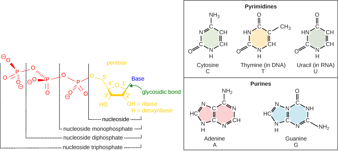
The nitrogenous bases found in nucleic acids include adenine and guanine (called purines) and cytosine, uracil, or thymine (called pyrimidines).

The purines have a double-ring structure with a six-membered ring fused to a five-membered ring.

Pyrimidines are smaller in size; they have a single six-membered ring structure.

(See Mnemonic on the right to help you remember).

Useful Mnemonic

 PURe As Gold!

Purines are Adenine and Guanine!

The remaining (T, C and U are Pyrimidines)

In molecular biology shorthand, we know the nitrogenous bases by their symbols A, T, G, C, and U.

DNA contains A, T, G, and C; whereas, RNA contains A, U, G, and C.

Building Nucleic Acid strands

The substrates for making DNA or RNA polymers are dNTPs (deoxyribonucleoside triphosphates- DNA) or NTPs  (for RNA).

Each DNA strand is built from dNTPs by the formation of a phosphodiester bond, catalyzed by DNA polymerase, between the 3’OH of one nucleotide and the 5’ phosphate of the next.

The result of this directional growth of the strand is that one end of the strand has a free 5’ phosphate and the other a free 3’ hydroxyl group (Figure 3.2). These are designated as the 5’ and 3’ ends of the strand.

During the formation of a nucleic acid polymer, the incoming nucleotides are added to a growing chain. During the reaction, the two outer phosphate groups  (beta and gamma) from the incoming dNTP are released. These two outer phosphates are called pyrophosphate after they are released.

RNA: Diverse Roles

We should take a moment to talk about RNA. “While they are both types of genetic material, RNA and DNA are rather different.

The chemical units of RNA are like those of DNA, except that RNA has the nucleotide uracil (U) instead of thymine (T). Unlike double-stranded DNA, RNA usually comes as only a single strand. And the nucleotides in RNA contain ribose sugar molecules in place of deoxyribose.

RNA is quite flexible—unlike DNA, which is a rigid, spiral-staircase molecule that is very stable. RNA can twist itself into a variety of complicated, three-dimensional shapes. RNA is also unstable in that cells constantly break it down and must continually make it fresh, while DNA is not broken down often. RNA’s instability lets cells change their patterns of protein synthesis very quickly in response to what’s going on around them.

Many textbooks still portray RNA as a passive molecule, simply a “middle step” in the cell’s gene-reading activities. But that view is no longer accurate. ” (1)

We will come back to this amazing molecule and its role in the regulation of gene expression and genetic medicine in later chapters.

3.3 Identity of DNA as Genetic Material

That eukaryotic cells contain a nucleus was understood by the late 19th century.  By then, histological studies had shown that nuclei contained largely proteins and DNA.  At around the same time, the notion that the nucleus contains genetic information was gaining traction.

However, DNA was thought to be a monotonous, repetitive string of nucleotides, which would not be useful for information storage. The prevailing hypothesis by Phoebus Levene was the “tetranucleotide hypothesis,” which postulated that DNA’s four bases are present in equal amounts and repeat over and over again along the chromosome in a fixed pattern.  On the other hand, as chains of up to 20 different amino acids, polypeptides and proteins had the potential for enough structural diversity to account for the growing number of heritable traits in a given organism. Thus, proteins over nucleic acids seemed more likely candidates for the molecules of inheritance.

The experiments you will read about here began around the start of World War I and lasted until just after World War 2.  During this time, we learned that DNA was no mere tetramer, but was in fact a long polymer.

This led to some very clever experiments that eventually forced the scientific community to conclude that DNA, not protein, was the genetic molecule, despite being composed of just four monomeric units.

3.3.1  Transforming Principle – Griffiths Experiments

in 1928, British bacteriologist Frederick Griffith reported the first demonstration of bacterial transformation—a process in which external DNA is taken up by a cell, thereby changing its morphology and physiology.

He had discovered three immunologically different strains of Streptococcus pneumonia (Types I, II, and III).  The virulent strain (Type III) was responsible for much of the mortality during the Spanish Flu (influenza) pandemic of 1918-1920.  This pandemic killed between 20 and 100 million people, many because the influenza viral infection weakened the immune system of infected individuals, making them susceptible to bacterial infection by Streptococcus pneumonia.

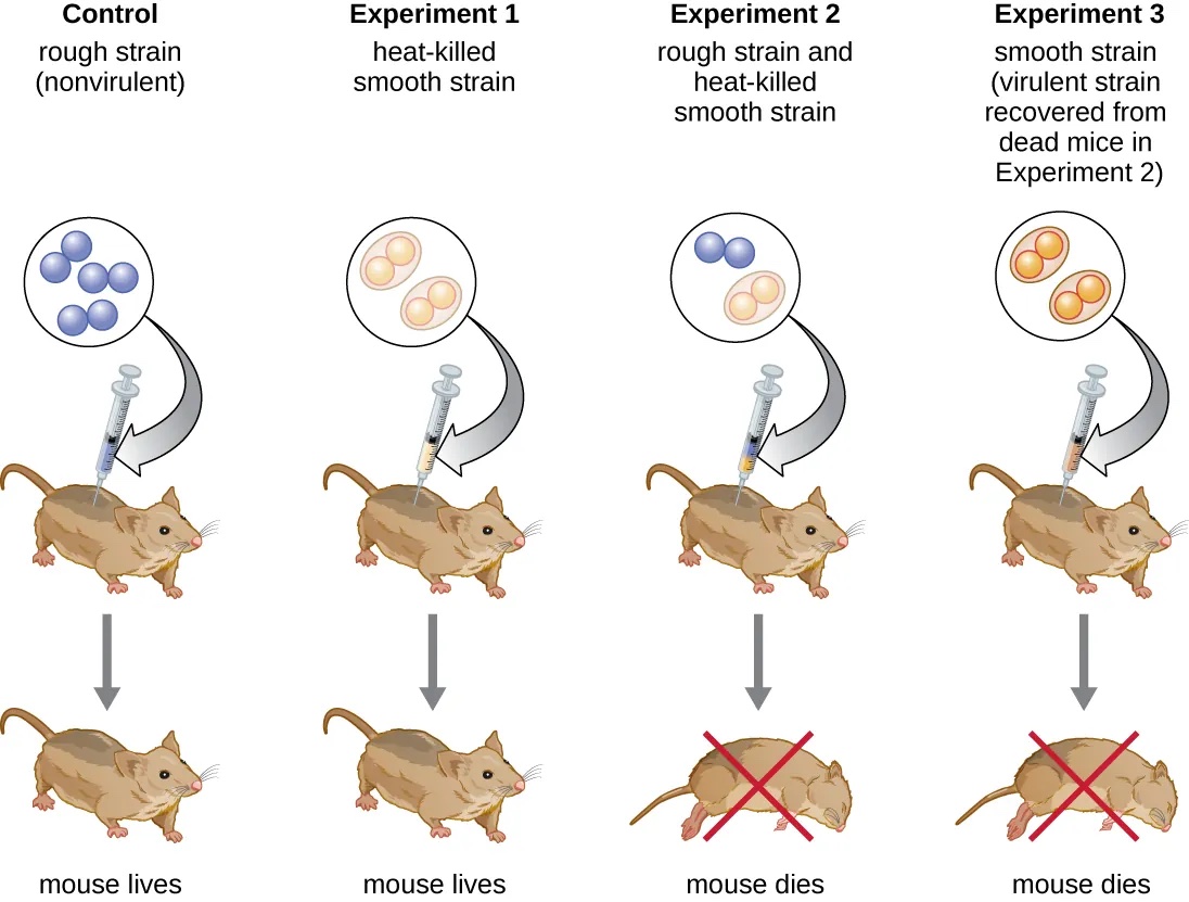
In the 1920s, Frederick Griffith was working with virulent wild-type (Type III) and benign (Type II) strains of S. pneumonia.  The two strains were easy to tell apart in Petri dishes because the virulent strain grew as morphologically smooth colonies, while the benign strain formed rough colonies.  For this reason, the two bacterial strains were called S  (smooth) and R (rough), respectively.

When Griffith injected the living S strain into mice, they died from pneumonia. In contrast, when Griffith injected the live R strain into mice, they survived. In another experiment, when he injected mice with the heat-killed S strain, they also survived. This experiment showed that the capsule alone was not the cause of death.

In the third set of experiments, a mixture of live R strain and heat-killed S strain were injected into mice, and—to his surprise—the mice died.

Upon isolating the live bacteria from the dead mouse, only the S strain of bacteria was recovered. When this isolated S strain was injected into fresh mice, the mice died. Griffith concluded that “information” had transferred from the heat-killed S strain into the live R strain, transforming it into the pathogenic S strain. He called this the transforming principle (Figure 3.3 ).

These experiments are now known as Griffith’s transformation experiments.

3.3.2 The Avery-MacLeod-McCarty and the Hershey-Chase experiments.

While Griffith didn’t know the chemical identity of his transforming principle, his experiments led to studies that proved DNA to be the stuff of genes.

With improved molecular purification techniques developed in the 1930s, O. Avery, C. MacLeod, and M. McCarty transformed R cells in vitro (that is, without the help of a mouse!),  ‘ a biochemical assay’ for transformation!

They isolated proteins and nucleic acids (RNA and DNA) from the S-strain, as these were possible candidates for the molecule of heredity.

They then used enzymes that specifically degraded each component and used the enzyme-treated mixture to transform the R strain.

They found that when DNA was degraded enzymatically, the resulting mixture was no longer able to transform the bacteria, whereas all of the other combinations were able to transform the bacteria.

This led them to conclude that DNA was the transforming principle.

WATCH: Whiteboard video

Attribution: This video is from The Explorer’s Guide to Biology (XBio) and is offered under a CC-BY-NC licensing agreement. For more information, see Ronald Vale’s Narrative on DNA Structure in The Explorer’s Guide to Biology (explorebiology.org/collections/genetics/dna-structure).

Although the experiments of Avery, McCarty, and McLeod had demonstrated that DNA was the informational component transferred during transformation, DNA was still considered to be too simple a molecule to carry biological information. Since this result stood against the dogma of the time, it was not readily accepted.

The decisive experiment, conducted by Martha Chase and Alfred Hershey in 1952, provided confirmatory evidence that DNA was indeed the genetic material and not proteins.

Hershey and Chase Experiments

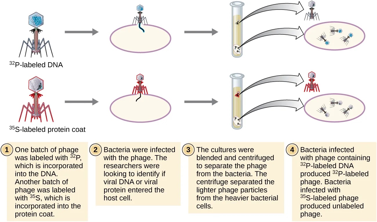
Chase and Hershey were studying a bacteriophage—a virus that infects bacteria.  Bacteriophages have a very simple structure: a protein coat called the capsid, and a nucleic acid core that contains the genetic material (either DNA or RNA).

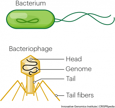
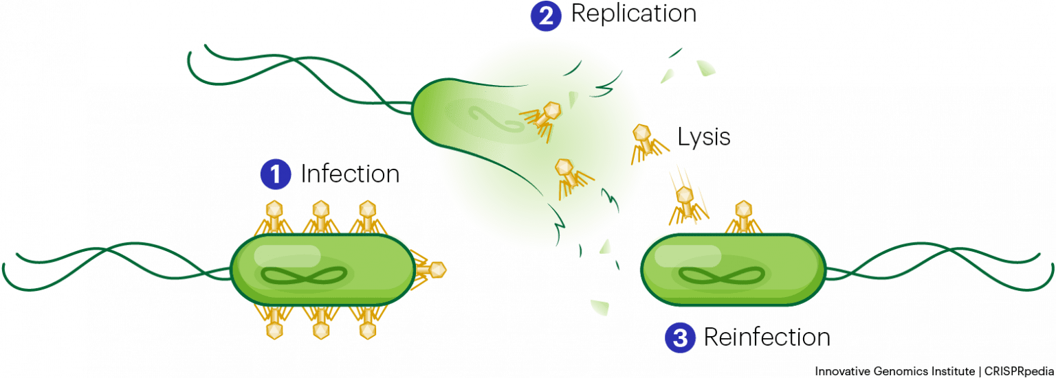
The bacteriophage infects the host bacterial cell by attaching to its surface, and then it injects its nucleic acids inside the cell.  The bacteria’s own protein machinery replicates the phage genome. The bacterium then follows the instructions in the phage DNA and generates more heads, tails, tail fibers, and other phage pieces which then assemble. Eventually, the host cell bursts (lyses), releasing a large number of bacteriophages. This is similar to a balloon popping. (see figure below)

Hershey and Chase selected radioactive elements that would specifically distinguish the protein from the DNA in infected cells.

They labeled one batch of phage with radioactive sulfur, ³⁵S, to label the protein coat. Another batch of phage was labeled with radioactive phosphorus, ³²P.

Because phosphorous is found in DNA, but not protein, the DNA and not the protein would be tagged with radioactive phosphorus. Likewise, sulfur is absent from DNA but is present in several amino acids such as methionine and cysteine.

Each batch of labeled phage was allowed to infect the cells separately. After infection, the phage bacterial suspension was put in a blender, which caused the phage coat to detach from the host cell. Cells exposed long enough for infection to occur were then examined to see which of the two radioactive molecules had entered the cell. The phage and bacterial suspension were spun down in a centrifuge. The heavier bacterial cells settled down and formed a pellet, whereas the lighter phage particles stayed in the supernatant. In the tube that contained phage labeled with ³⁵S, the supernatant contained the radioactively labeled phage, whereas no radioactivity was detected in the pellet.

Around this same time, Austrian biochemist Erwin Chargaff examined the content of DNA in different species. He found that the relative concentrations of the four nucleotide bases varied from species to species, but not within tissues of the same individual or between individuals of the same species.

He also discovered something unexpected: the amount of adenine equaled the amount of thymine, and the amount of cytosine equaled the amount of guanine (that is, A = T and G = C). Different species had equal amounts of purines (A+G) and pyrimidines (T + C), but different ratios of A+T to G+C. These observations became known as Chargaff’s rules.

Chargaff’s findings proved immensely useful when Watson and Crick were getting ready to propose their DNA double helix model!

Key Takeaways

1. DNA was first isolated from white blood cells by Friedrich Miescher, who called it nuclein because it was isolated from nuclei.
2. Frederick Griffith’s experiments with strains of Streptococcus pneumoniae provided the first hint that DNA may be the transforming principle.
3. Avery, MacLeod, and McCarty showed that DNA is required for the transformation of bacteria.
4. Later experiments by Hershey and Chase using bacteriophage T2 proved that DNA is the genetic material.
5. Chargaff found that the ratio of A = T and C = G, and that the percentage content of A, T, G, and C is different for different species.

Did I get this?

3.4 DNA Structure: The Double Helix

When DNA was accepted as the stuff of genes, the next questions were

•  What did DNA look like?
• How did its structure account for its ability to encode and reproduce life?

While the nature of DNA and its composition of 4 nucleotides had been known for some time, it became mandatory to explain how such a “simple molecule” could inform the thousands of proteins necessary for life.

The answer to this question was to lie at least in part in an understanding of the physical structure of DNA, made possible by the advent of X-Ray Crystallography.

3.4.1 Wilkins, Franklin, Watson & Crick – DNA Structure Revealed.

William Astbury demonstrated that high molecular weight DNA had just such a regular structure.  His imaging suggested DNA was a linear polymer of stacked bases (nucleotides), each nucleotide separated from the next by 0.34 nm.

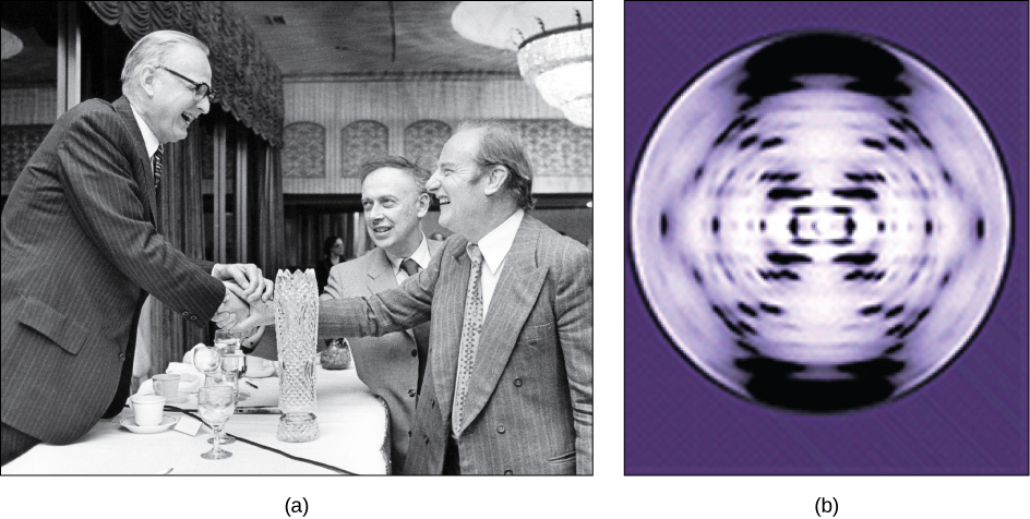
Maurice Wilkins, an English biochemist, was the first to isolate highly pure, high molecular weight DNA.  Working in Wilkins laboratory, Rosalind Franklin was able to crystalize this DNA and produce very high-resolution X-Ray diffraction images of the DNA crystals.  Franklin’s most famous (and definitive) image was “Photo 51” (Fig. 3.5 -b).

Franklin’s image confirmed Astbury’s 0.34 nm repeat dimension and revealed two more numbers, 3.4 nm, and 2 nm, reflecting additional repeat structures in the DNA crystal.  When James Watson and Francis Crick got hold of these numbers, they used them along with other data to build DNA models out of nuts, bolts, and plumbing.

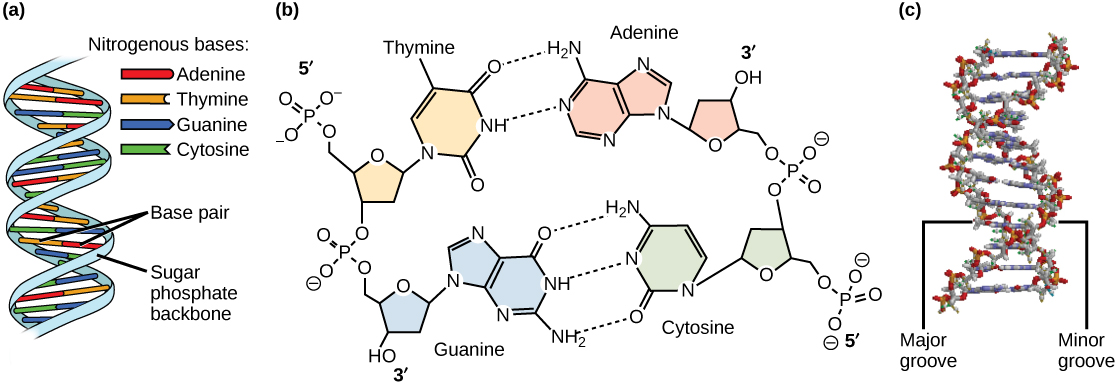
Watson and Crick proposed that DNA is made up of two strands that are twisted around each other to form a right-handed helix. Base pairing takes place between a purine and pyrimidine on opposite strands, so that A pairs with T, and G pairs with C (suggested by Chargaff’s Rules).

Thus, adenine and thymine are complementary base pairs, and cytosine and guanine are also complementary base pairs.

 

The base pairs are stabilized by hydrogen bonds: adenine and thymine form two hydrogen bonds and cytosine and guanine form three hydrogen bonds.

The two strands are anti-parallel in nature; that is, the 3′ end of one strand faces the 5′ end of the other strand. The sugar and phosphate of the nucleotides form the backbone of the structure, whereas the nitrogenous bases are stacked inside, like the rungs of a ladder.

Each base pair is separated from the next base pair by a distance of 0.34 nm, and each turn of the helix measures 3.4 nm. Therefore, 10 base pairs are present per turn of the helix. The diameter of the DNA double-helix is 2 nm, and it is uniform throughout.

Only the pairing between a purine and pyrimidine and the antiparallel orientation of the two DNA strands can explain the uniform diameter.

The twisting of the two strands around each other results in the formation of uniformly spaced major and minor grooves or indentations on the sides of the helix (Figure 3.6).

Protein-DNA interactions occur in these spaces. The grooves expose the edges of the bases to the external environment, making them accessible for protein binding.

The nature of the atoms that are exposed in the grooves forms a type of code or pattern that proteins that bind DNA use to recognize sequences without needing to pry open the DNA helix!   Discrimination of the different sequences must be made by having access to the bases inside the structure since the backbone structure is common to all sequences of DNA.

[See the video below on DNA Structure and Lecture Videos in the playlist for further explanation]

 

 

TIME to THINK:

To function as the molecule of inheritance the molecule should be stable, store information (vasts amount to account for all the variability), capacity to change (to account for evolution and diversity of life), and faithfully replicate (to account for the continuity of life and perpetuation of species).  It is not surprising that Proteins were initially favored over DNA as being the molecule of inheritance given the tall order.

However, once Watson and Crick proposed and published their model of DNA as a double helix the answer was obvious. The structure perfectly suited its function!

Think about how the simple elegant structure and features of the double helix can fulfill the requirements needed for a molecule of inheritance. Jot down your thoughts.

Watch this video on DNA structure:

---

Before you continue you should

1. Watch the Lecture videos that cover the material above.
2. Complete any exercises, or problems if assigned.

---

3.5 Analysis of Nucleic Acids

When Watson and Crick submitted their historic one-page paper on the model DNA structure they included a provocative message.

“It has not escaped our notice that the specific pairing that we have postulated immediately suggests a possible copying mechanism for the genetic material.”

While the exact mechanism of replication was eventually experimentally proven, fundamental to the process was the separation of DNA strands. Experimentally scientists had shown that when DNA molecule was heated or treated with chemicals (like Urea) the viscosity of the DNA solution dropped.

The forces holding duplexes together include hydrogen bonds between the bases of each strand that, like the hydrogen bonds in proteins, can be broken with heat or urea. (Another important stabilizing force for DNA arises from the stacking interactions between the bases in a strand.)

The separation of strands of the double helix into single strands is Denaturation.

Single strands absorb light at 260 nm more strongly than double strands. This is known as the hyperchromic effect (Figure 3. ) and is a consequence of the disruption of interactions among the stacked bases. The changes in absorbance allow one to easily follow the course of DNA denaturation.

Denatured duplexes can readily renature when the temperature is lowered below the “melting temperature” or Tm, the temperature at which half of the DNA strands are in duplex form. Under such conditions, the two strands can re-form hydrogen bonds between the complementary sequences, returning the duplex to its original state.

In most organisms, the Tm of the chromosomal DNA ranges from 85-100 degrees C. It is possible to determine the composition of the DNA experimentally from its Tm because the Tm of DNA is directly proportional to the GC content of the DNA.

For DNA, this principle of strand separation and renaturation (also called hybridization or annealing) are important for many techniques- and most importantly will feature again when we learn about polymerase chain reaction (PCR).

Historically, the separation of DNA and subsequent renaturation was used to assess the complexity of the genome, % GC content, and similarity between sequences.

Did I get this?

Agarose Gel Electrophoresis

DNA molecules can be separated by size and visualized using electrophoresis. The principle is similar to that discussed for proteins with a few exceptions.

1. Since DNA is naturally negatively charged there is no need to use detergents like SDS. DNA molecule migrates towards the positively charged electrode (cathode).

2. The polymer used for DNA electrophoresis is Agarose (hence the name).

3. Agarose gels are usually poured and run horizontally.

The rate of migration is directly dependent on the ability of each DNA molecule to worm or wiggle its way through the sieving matrix.  The largest macromolecules have the most difficult time navigating through the gel, whereas the smallest macromolecules slip through it the fastest.

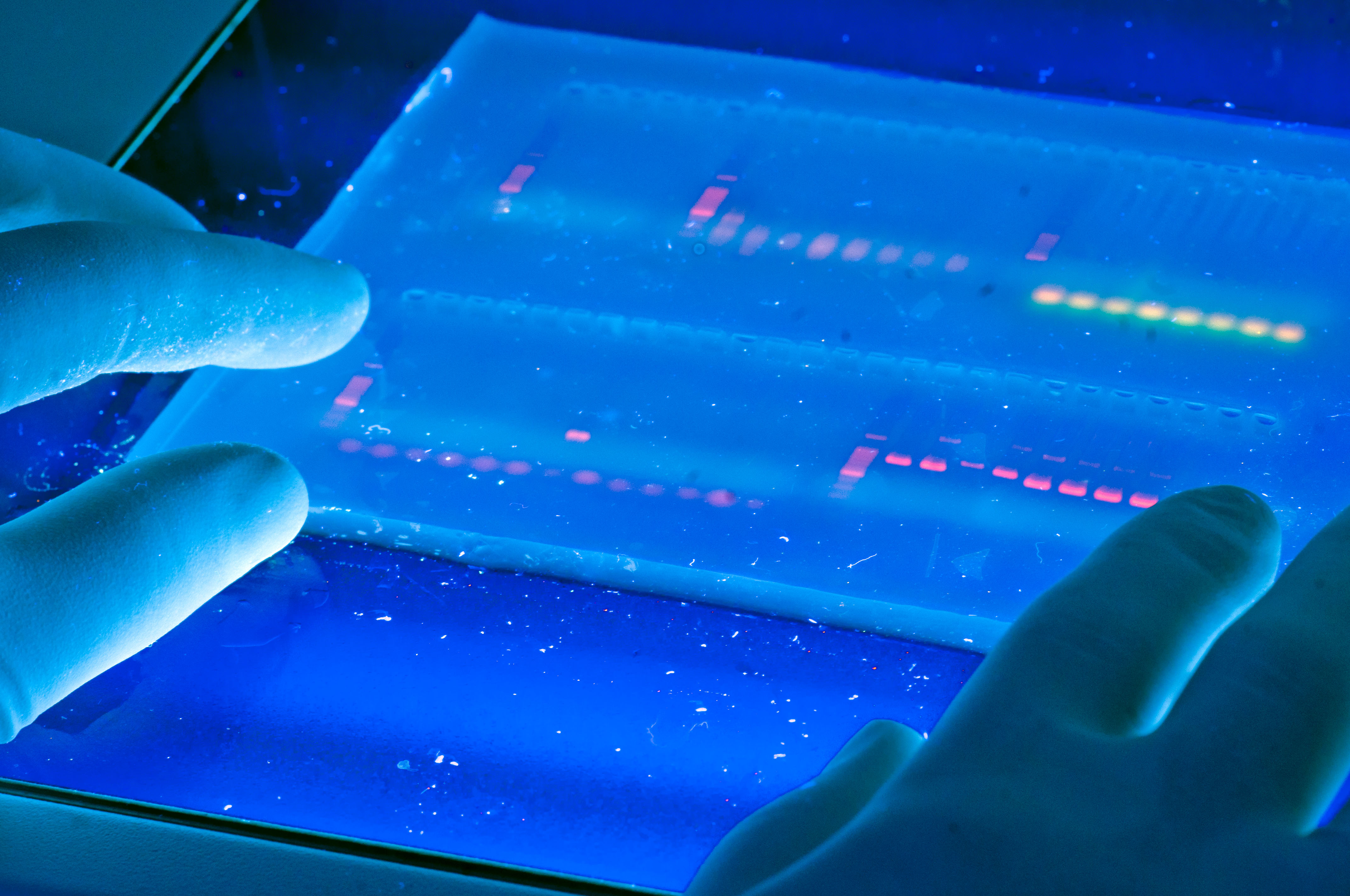
4. Visualization of DNA occurs by using a fluorescent dye ethidium bromide.

This compound contains a planar group that intercalates between the stacked bases of DNA. The dye is usually incorporated into the gel and running buffer, the stain is visualized by irradiating with a UV light source (i.e. using a transilluminator) and photographing with polaroid film. (Figure 3.7)

Ethidium being a DNA intercalating agent is a powerful mutagen! There are newer safer, less toxic alternative DNA gel stains developed in recent years. Such stains typically have a detection limit that falls in the range of 1-5 ng DNA/band.

5. Reference DNAs of known sizes are alongside the samples (DNA ladders).

This allows ones to determine the sizes of the DNA fragments in the sample.

It is useful to note that, by convention, DNA fragments are not described by their molecular weights (unlike proteins), but by their length in base-pairs( bp) or kilobases (kb).

3.6 From Genes to Genomes

We use the word “genome” to describe all of the genetic material of the cell. That is, a genome is an entire sequence of nucleotides in the DNA that is in all of the chromosomes of a cell. When we use the term genome without further qualification, we are generally referring to the chromosomes in the nucleus of a eukaryotic cell.

As you know, eukaryotic cells have organelles like mitochondria and chloroplasts that have their own DNA. These are referred to as the mitochondrial or chloroplast genomes to distinguish them from the nuclear genome.

Starting in the 1980s, scientists began to determine the complete sequence of the genomes of many organisms, in the hope of better understanding how the DNA sequence specifies cellular functions.

The Human Genome Project (HGP) was one of the great feats of exploration in history. Rather than an outward exploration of the planet or the cosmos, the HGP was an inward voyage of discovery led by an international team of researchers looking to sequence and map all of the genes — together known as the genome — of members of our species, Homo sapiens.

Beginning on October 1, 1990, and completed in April 2003, the HGP gave us the ability, for the first time, to read nature’s complete genetic blueprint for building a human being.

The technological advances in the ability to sequence DNA that were a direct result of this colossal endeavor resulted in a new field of study: Genomics; the comprehensive study of whole sets of genes and their interactions.

The results are deposited into publicly available databases. You can find many of them at the National Center for Biotechnology Information.

The number of available, completely sequenced genomes numbers in the tens of thousands—over 2,000 eukaryotic genomes, over 600 archaeal genomes, and nearly 12,000 bacterial genomes. Tens of thousands of more genome sequencing projects are in progress.

As the sequence databases compile ever more information, the fields of computational biology and bioinformatics have arisen, to analyze and organize the data in a way that helps biologists understand what the information in DNA means in the cellular context.

With this many genome sequences available— scientists have been asking many questions about what we see in these genomes. What patterns are common to all genomes? How many genes are encoded in genomes? How are these organized? How many different types of features can we find? How different are the genomes from one another?

3.6.1 Diversity of genomes

Diversity of sizes, number of genes, and chromosomes

Let’s start by examining the range of genome sizes. In the table below, we see a sampling of genomes from the database. We can see that the genomes of free-living organisms range tremendously in size. The smallest known genome is encoded in 580,000 base pairs while the largest is 150 billion base pairs—for reference, recall that the human genome is 3.2 billion base pairs. That’s a huge range of sizes.

 

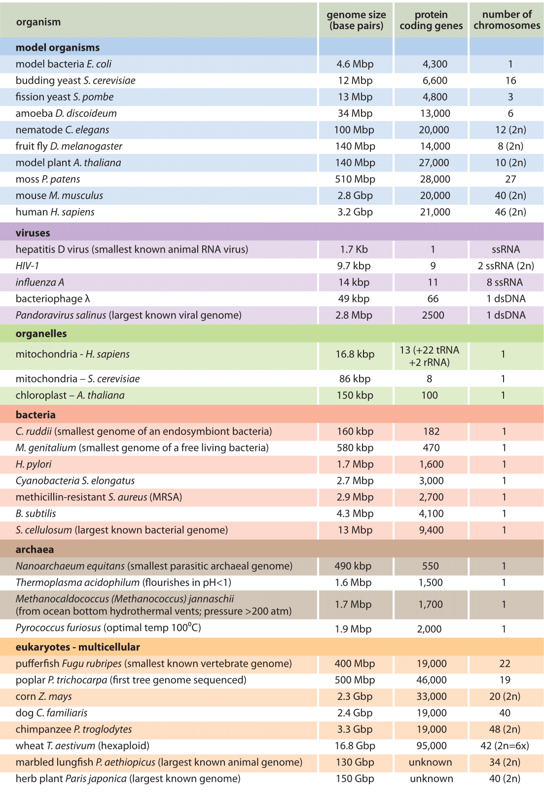
Notice the genome sizes of Prokaryotes in base pairs and compare them with those of multicellular organisms. At first glance, we see that the overall genomes of viruses, archaea, bacteria (and some unicellular eukaryotes) are smaller.

A common-sense assumption about genomes would be that if genes specify proteins, then the more proteins an organism made, the more genes it would need to have, and thus, the larger its genome would be.

However, when we begin to see how much of the genome is devoted to protein-coding genes a different story emerges that indicates that in fact there is NO direct relationship between the complexity of an organism and the size of its genome.

Comparing the pufferfish genome to the chimpanzee genome, we note that they encode roughly the same number of genes (19,000), but they do so on dramatically differently sized genomes—400 million base pairs versus 3.3 billion base pairs, respectively.

That implies that the pufferfish genome must have much less space between its genes than what might be expected to be found in the chimpanzee genome. Indeed, this is the case, and the difference in gene density is not unique to these two genomes.

In fact, we can broadly categorize genomes as being either:

• Small, compact genomes like those of viruses, archaea, and bacteria or
• Large and expanded where the bulk of the genome is non-coding.

To understand how this could be true, it is necessary to recognize that while genes are made up of DNA, all DNA does not consist of genes (for purposes of our discussion, we define a gene as a section of DNA that encodes an RNA or protein product).

One of the surprising findings of the human genome data was that less than 2% of the total DNA seems to be the sort of coding sequence that directs the synthesis of proteins.  For many years, non-coding DNA in genomes was believed to be useless and was described as “junk DNA” although it was perplexing that there seemed to be so much “useless” sequence. Recent discoveries have, however, demonstrated that much of this so-called junk DNA plays important roles in evolution, as well as in the regulation of gene expression

What is all the “extra stuff” in the eukaryotic genomes?

Introns

We know that even coding regions in our DNA are interrupted by non-coding sequences called introns. This is true of most eukaryotic genomes. An examination of genes in eukaryotes shows that non-coding intron sequences can be much longer than the coding sections of the gene, or exons. Most exons are relatively small, and code for fewer than a hundred amino acids, while introns can vary in size from several hundred base pairs to many kilobase pairs (thousands of base pairs) in length. For many genes in humans, there is much more of intron sequence than coding (a.k.a. exon) sequence. Intron sequences account for roughly a quarter of the genome in humans.

Introns get removed (spliced) after transcription, something you will learn in upcoming chapters.

Regulatory Sequences

What other kinds of non-coding sequences are there? One function for some DNA sequences that do not encode RNA or proteins is in specifying when and to what extent a gene is used or expressed. Such regions of DNA are called regulatory regions and each gene has one or more regulatory sequences (promoters and enhancer sequences) that control its expression. However, regulatory sequences do not account for all the rest of the DNA in our genomes, either.

Repetitive DNA

More than 50% of the genome and the ‘intergenic’ regions consist of highly repetitive sequences. Some of these are found in regions of the DNA that go on to form structural markers of chromosomes like centromeres and telomeres.

Genome-Wide or Interspersed Repeats

Many of the repetitive sequences are known to be transposable elements (transposons), sections of DNA that can move around within the genome. Sometimes referred to as “jumping genes” these transposable elements can move from one chromosomal location to another, either through a simple “cut and paste” mechanism that cuts the sequence out of one region of the DNA and inserts it into another location or through a process called retrotransposition involving an RNA intermediate. These are dispersed throughout the genome. These repetitive DNA elements are further subdivided into two categories based on their length.

Tandem Repeats

In contrast to the repeats that are dispersed, tandem repeats are placed next to each other in an array. Amongst these are short tandem repeats or STRs. Each repeat is a unique DNA sequence that ranges from 2 to 6 bp repeated over and over, eg GACA GACA GACA.

The number of repeats is variable in different individuals and since these are inherited they are the basis of forensic genetic analysis to generate a DNA profile of an individual.

Interestingly the fact that our genomes consisted of highly repetitive DNA sequences was known as early as the ’60s by denaturation and renaturation experiments!

See below for an example of the kind of scientific application connected with concepts discussed earlier.

Link to Learning

Go to: http://www.dnaftb.org/31/index.html

Click through the Animation tab to learn about early experiments revealing the presence of repetitive DNA in genomes.

ENCODE

The sequencing phase of the Human Genome Project provided a massive data set of ordered bases but did not show where genes begin or end or what they do.

The project ENCODE or the Encyclopedia of DNA Elements ( ENCODE ) set out to identify all functional elements in the human and mouse genome sequences – this includes protein‐coding genes, non‐protein‐coding genes, transcriptional regulatory elements, and sequences that mediate chromosome structure and dynamics. The ENCODE Project started in 2003 with the ENCODE Pilot Project, which focused on 1% of the human genome and is now in its fourth phase.

Key Takeaways

Watch the Key Takeaways lecture videos related to this topic on your CANVAS page.

References and Attributions

This chapter contains material taken from the following CC-licensed content. Changes include rewording, removing paragraphs, and replacing them with original material.

• (1) Introduction and RNA- Diverse Roles  From the New Genetics is available online at: http://publications.nigms.nih.gov/thenewgenetics. NIH Publication No. 10-662. Revised April 2010. (US Government Work)
• Ahern K, Rajagopal I and Tan T. (2013). Biochemistry Free for All (Version 1.3). Licensed under a Creative Commons Attribution-NonCommercial 4.0 International License. The entire textbook is available for free from the authors at http://biochem.science.oregonstate.edu/content/biochemistry-free-and-easy.
• ” DNA, Chromosomes and Chromatin” by Gerald Bergstom, LibreTexts is licensed under CC BY. The chapter can be found online at https://bio.libretexts.org/@go/page/16463. The entire textbook Basic Cell and Molecular Biology: What We Know & How We Found Out – 4e can be found at https://open.umn.edu/opentextbooks/textbooks/cell-and-molecular-biology-2e-what-we-know-how-we-found-out

Section 3.6 From Genes to Genomes:

• Genomes: a Brief Introduction. (2019, June 2). https://bio.libretexts.org/@go/page/9388
• “Genes and Genomes” by Kevin Ahern, Indira Rajagopal, & Taralyn Tan, LibreTexts is licensed under CC BY-NC-SA.  The entire textbook is available free from the authors at http://biochem.science.oregonstate.edu/content/biochemistry-free-and-easy

Images

Figure images without any attribution in the caption are licensed under CC-BY 4.0 by OpenStax. Located at: https://openstax.org/books/biology-2e/pages/14-1-historical-basis-of-modern-understanding. Access for free at https://openstax.org/books/biology-2e/pages/1-introduction

Figure 3.3 and 3.4 Parker, Nina , Mark Schneegurt , Anh-Hue Thi Tu, Philip Lister, and Brian  M Foster. “Using Microbiology to Discover Secrets of Life.” In Microbiology . Houston, Texas : OpenStaxn.d.

Access for free at https://openstax.org/books/microbiology/pages/1-introduction