
2 Chapter 2. Atmosphere Ocean Interactions
Ocean circulation
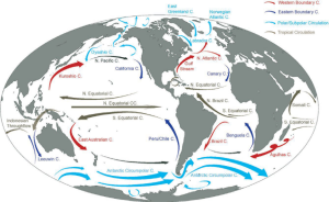
Seawater flows along the horizontal plane and in the vertical direction. Typical speeds of the horizontal flow or currents are 0.01-1.0 m/s (about 0.4-3.6 km/h or 0.3-2.2 mi/h); vertical speeds within the stratified ocean are much smaller, closer to 0.001 m/s (0.01 mi/h). Two forces produce the non-tidal ocean currents: a) the wind exerting a stress on the sea surface and b) buoyancy (heat and freshwater) fluxes between the ocean and atmosphere that alter the density of the surface water. The former induces what we call the wind driven ocean circulation (ocean surface currents, such as Gulf Stream), the latter the thermohaline circulation (deep ocean circulation). The wind driven circulation is by far the more energetic but for the most part resides in the upper kilometer of the ocean. The sluggish thermohaline circulation reaches in some regions to the sea floor, and is associated with ocean overturning linked to the formation and spreading of the major water masses of the global ocean, such as North Atlantic Deep Water and Antarctic Bottom Water.
Ekman Transport (Spiral)
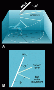
Norwegian explorer Fridtjof Nansen (1861-1930) was interested in ocean currents in polar seas. In 1893, he allowed his 39-m (128-ft) wooden ship, the Fram, to freeze into Arctic pack ice about 1100 km (680 mi) south of the North Pole. His goal was to drift with the ice and get to the North Pole. The Fram drifted with pack ice for 35 months and came within 394 km (244 mi) of the North Pole. As the Fram slowly drifted with the ice, Nansen noticed that the direction of ice and ship movement was consistently 20 to 40 degrees to the right of the prevailing wind direction.
Swedish physicist V. Walfrid Ekman (1874-1954) used Nansen’s idea and observations and described Ekman Spiral model mathematically in 1905. Because of Earth’s rotation, the shallow layer of surface water set in motion by the wind is deflected to the right of the wind direction in the Northern Hemisphere and to the left of the wind direction in the Southern Hemisphere (Coriolis Effect). The Ekman spiral indicates that each successive layer moves more toward the right of the overlying layer’s and at a slower speed. The Ekman spiral predicts net water movement through a depth of about 100 to 150 m (330 to 500 ft) at 90 degrees to the wind direction, to the right in northern hemisphere and to the left in southern hemisphere.
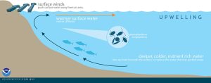
As the wind varies from place to place, Ekman transport can produce divergence (upwelling) or convergence (downwelling) of surface water. Upwelling occurs when water rises up from beneath the surface to replace the water that was pushed away by winds. This process may occur in the open ocean and along coastlines. Water that rises to the surface as a result of upwelling is typically colder and is rich in nutrients. These nutrients induce high biological productivity and abundance of plankton, which attract fish and other life in ocean, making upwelling areas great fishing grounds. In other regions of the ocean downwelling occurs when wind causes water to build up along a coastline and the surface water eventually sinks toward the bottom.
The surface ocean layer is less dense (more buoyant) than the deeper layers, therefore a spatially variable Ekman transport field acts to redistribute the buoyant surface water: thinning the buoyancy surface layer in divergence regions, thickening the buoyant surface layer in convergence regions. As the ocean is in hydrostatic equilibrium, the redistribution of the buoyant surface layer induces sea level “valleys” in divergent regions and “hills” in convergence regions. While these hills and valleys amount to only a 1.5 meter in amplitude, they are sufficient to induce horizontal pressure gradients which initiate the wind driven circulation following the geostrophic balance concept. The ocean currents are for the most part geostrophic, meaning that the Coriolis Effect balances the horizontal pressure gradients. The wind driven circulation is characterized by large clock-wise (northern hemisphere) and counter clock-wise (southern hemisphere) flowing gyres, such as the subtropical and subpolar gyres.
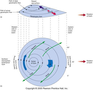
Figure 4 details.
A cross-sectional and map view of a large ocean gyre show how water piles up in the center and how the Coriolis Effect creates western intensification. (Source: Pearson Prentice Hall)
In both hemispheres, the currents making up the western side of the gyre are much more intense than the currents on the eastern side. This phenomenon is known as western intensification, and it is also due to the Coriolis Effect. The same volume of water must pass through both the east and west sides of the gyre. In the western gyre currents, that volume is passing through a narrower area, so the current must travel faster in order to transport the same amount of water in the same amount of time. On the eastern side of the gyre the current is much wider, so the flow is slower. For example, the Gulf Stream – a western boundary current in Atlantic Ocean – is only 50-100 km wide, but deep (up to 1.5 km), and relatively fast (6.4-9 km/hr), while on the eastern side of gyre is Canary Current, which is about 1000 km wide, but shallow (0.5 km) and very slow (0.7-1 km/hr).
Thermohaline and global overturning Circulation
In the Earth’s polar regions ocean water gets very cold, forming sea ice. As a consequence the surrounding seawater gets saltier, because when sea ice forms, the salt is left behind. As the seawater gets saltier, its density increases, and it starts to sink. Surface water is pulled in to replace the sinking water, which in turn eventually becomes cold and salty enough to sink. This initiates the deep-ocean currents (thermohaline circulation) driving the global conveyer belt. The thermohaline circulation engages the full volume of the ocean into the climate system, by allowing all of the ocean water to ‘meet’ and interact directly with the atmosphere (on a time scale of 100-1000 years).
The global overturning circulation is a system of ocean currents that moves heat, freshwater, and carbon around the Earth. There is a surplus of heat in the tropics relative to the poles due to incoming solar radiation. The Atlantic Ocean plays a key role in redistributing this heat, as well as salt, dissolved oxygen, nutrients, and carbon throughout the global climate system. Variations in the strength of the Atlantic Ocean overturning circulation have direct societal impacts on coastal sea levels, marine heat waves, extreme weather events, and shifts in regional weather and global climate.
![A simplified 2-d illustration of the Atlantic Meridional Overturning Circulation (AMOC) and its impact on the mean air-sea flux and transport of heat, oxygen (O2), anthropogenic (CANTH) and natural carbon (CNAT). High latitude basins such as the North Atlantic are regions of strong heat loss and uptake of CANTH, CNAT and O2. Upwelling in the Southern Ocean leads to simultaneous release of CNAT, uptake of CANTH and O2 ventilation as the upwelled deep waters are low in O2 and rich in Dissolved Inorganic Carbon (DIC). The equatorial zone is a region of intense upwelling of cold, nutrient and DIC-rich waters, driving enhanced uptake of heat, biological production and thermal outgassing of O2, and strong release of CNAT. [AABW=Antarctic Bottom Water; NADW=North Atlantic Deep Water; IDW=Indian Deep Water; PDW=Pacific Deep Water; AAIW=Antarctic Intermediate Waters; SAMW=Subantarctic Mode Water]](https://iu.pressbooks.pub/app/uploads/sites/1390/2023/02/AMOC-300x153.png)
Figure 5 Details.
A simplified 2-d illustration of the Atlantic Meridional Overturning Circulation (AMOC) and its impact on the mean air-sea flux and transport of heat, oxygen (O2), anthropogenic (CANTH) and natural carbon (CNAT). High latitude basins such as the North Atlantic are regions of strong heat loss and uptake of CANTH, CNAT and O2. Upwelling in the Southern Ocean leads to simultaneous release of CNAT, uptake of CANTH and O2 ventilation as the upwelled deep waters are low in O2 and rich in Dissolved Inorganic Carbon (DIC). The equatorial zone is a region of intense upwelling of cold, nutrient and DIC-rich waters, driving enhanced uptake of heat, biological production and thermal outgassing of O2, and strong release of CNAT. [AABW=Antarctic Bottom Water; NADW=North Atlantic Deep Water; IDW=Indian Deep Water; PDW=Pacific Deep Water; AAIW=Antarctic Intermediate Waters; SAMW=Subantarctic Mode Water] (Source: B. Delorme and Y. Eddebbar, 2017).
Teleconnections
Changes in the atmosphere in one place can affect weather over 1000 miles away. These patterns are called teleconnections. Teleconnection patterns are caused by changes in the way air moves around the atmosphere. The changes may last from a few weeks to many months. Teleconnection patterns are natural and they include ENSO, AO, NAO, PDO, PNA, MJO, etc.
ENSO – El Niño Southern Oscillation
The El Niño-Southern Oscillation (ENSO) is a recurring climate pattern involving changes in the temperature of waters in the central and eastern tropical Pacific Ocean. On periods ranging from about three to seven years, the surface waters across a large swath of the tropical Pacific Ocean warm or cool by anywhere from 1°C to 3°C, compared to normal. This oscillating warming and cooling pattern, referred to as the ENSO cycle, directly affects rainfall distribution in the tropics and can have a strong influence on weather across the United States and other parts of the world. El Niño (positive) and La Niña (negative) are the extreme phases of the ENSO cycle; between these two phases is a third phase called ENSO-neutral.
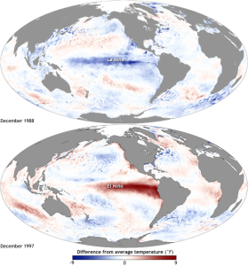
Figure 6 Details.
Maps of sea surface temperature anomaly in the Pacific Ocean during a strong La Niña (top, December 1988) and a strong El Niño (bottom, December 1997). (Source: NOAA Climate.gov)
El Niño: A warming of the ocean surface, or above-average sea surface temperatures (SST), in the central and eastern tropical Pacific Ocean. Over Indonesia, rainfall tends to become reduced while rainfall increases over the central and eastern tropical Pacific Ocean. The low-level surface winds, which normally blow from east to west along the equator (“Trade winds”), instead weaken or, in some cases, start blowing the other direction. In general, the warmer the ocean temperature anomalies, the stronger the El Niño (and vice-versa).
La Niña: A cooling of the ocean surface, or below-average sea surface temperatures (SST), in the central and eastern tropical Pacific Ocean. Over Indonesia, rainfall tends to increase while rainfall decreases over the central and eastern tropical Pacific Ocean. The normal easterly winds (“Trade Winds”) along the equator become even stronger. In general, the cooler the ocean temperature anomalies, the stronger the La Niña (and vice-versa).
ENSO Neutral: Neither El Niño or La Niña. Often tropical Pacific SSTs are generally close to average. However, there are some instances when the ocean can look like it is in an El Niño or La Niña state, but the atmosphere is not playing along (or vice versa).
Arctic Oscillation (AO)
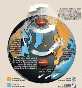
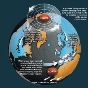
The Arctic Oscillation (AO) is a large scale mode of climate variability which is characterized by winds circulating counterclockwise around the Arctic at around 55°N latitude. When the AO is in its positive phase, a ring of strong winds circulating around the North Pole acts to confine colder air across polar region. This belt of winds becomes weaker and more distorted in the negative phase of the AO, which allows an easier southward penetration of colder, arctic air masses (Polar Vortex that sometimes sits above Great Lakes) and increased storminess into the mid-latitudes.
North Atlantic Oscillation (NAO)
The North Atlantic Oscillation (NAO) index is based on the surface sea-level pressure difference between the Subtropical (Azores) High and the Subpolar (Iceland) Low. The NAO phases are associated with basin-wide changes in the intensity and location of the North Atlantic jet stream and storm track, and in changes in temperature and precipitation patterns in eastern North America and western and central Europe. Positive phases of the NAO tend to be associated with above-normal temperatures in the eastern United States and across northern Europe and below-normal temperatures in Greenland and across southern Europe and the Middle East. They are also associated with above-normal precipitation over northern Europe and Scandinavia and below-normal precipitation over southern and central Europe. Opposite patterns of temperature and precipitation anomalies are typically observed during negative phases of the NAO. The NAO exhibits considerable inter seasonal and inter annual variability, and prolonged periods (several months) of both positive and negative phases of the pattern are common.
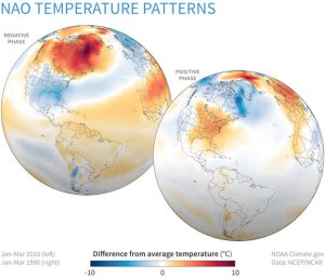
Figure 8 Details.
Late winter temperatures compared to the 1981-2010 average when the North Atlantic Oscillation (NAO) was strongly negative (top, Jan-March 2010) and when it was strongly positive (bottom, January-March 1990). (Source: NOAA, Climate.gov).
Pacific Decadal Oscillation (PDO)
The Pacific Decadal Oscillation (PDO) is a long-term ocean fluctuation of the Pacific Ocean. The ‘cool’ (negative) phase PDO is characterized by a cool wedge of lower than normal sea-surface ocean temperatures in the eastern equatorial Pacific and a warm horseshoe pattern of higher than normal sea-surface temperatures in the north, west and southern Pacific. In the ‘warm’ (positive) phase PDO, the west Pacific Ocean becomes cool and the wedge in the east warms. Unlike ENSO, the PDO isn’t one climate phenomenon. What we call the PDO is instead an aggregation of mostly independent processes. If ENSO is an ice cream flavor, the PDO is climate Neapolitan — a combo of different individual processes which influence a broader area. The three things that make up the PDO are: Aleutian Low, Reemergence of Sea Surface Temperatures (SST) and Kuroshio Sea Current.
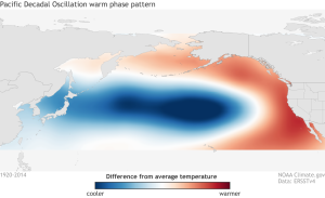
Figure 9 Details.
Sea surface temperature (SST) anomaly pattern associated with the positive (warm) phase of the PDO. Red shading indicates where SSTs are above average, and blue shading shows where SSTs are below average. (Source: M. Newman, NOAA Climate.gov)
The Aleutian Low is an area of low atmospheric pressure off the Aleutian Islands. If the Aleutian low is stronger-than-average, unusually strong southerly winds on the eastern side of the low run along the west coast of North America, warming the coastal waters by reducing the amount of cold water that normally upwells from depth. On the western side of a strong Aleutian low, the northerly winds and the stormy conditions help to churn up the water increasing the amount of cold water at the surface, and leading to below-normal sea surface temperature anomalies. The opposite is true for a weaker-than-average or non-existent Aleutian low. El Niño generally leads to a stronger-than-average Aleutian Low during winter while La Niña leads to a weaker Aleutian Low. Thus, one major influence on the PDO is the state of ENSO!
Pacific-North American (PNA) Teleconnection Pattern
The Pacific North American oscillation (PNA) is an alternating pattern of anomalous air pressure at four locations over the Pacific Ocean and North America, which correlate with regional temperature and precipitation anomalies across North America. A pattern of higher-than-average pressure in the vicinity of Hawaii and over the mountainous region of western North America, and lower-than-average pressure south of Alaska and over the southeastern United States defines the positive phase of PNA. This pressure pattern enhances the strength of the mid-latitude jet stream as it moves over the Pacific Ocean from eastern Asia. This situation increases the likelihood of above-average temperatures over western Canada and the western U.S. states, and below-average temperatures across south-central and southeastern U.S. states. In winter, the positive phase is also associated with below-average precipitation in the Pacific Northwest and across the eastern half of the United States.
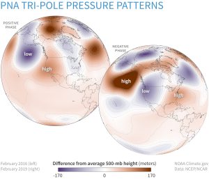
Figure 10 Details.
Air pressure in the lower atmosphere compared to the 1981-2010 average during February 2016 (left), when the PNA was positive, and in February 2019 (right), when it was negative. (Source: NOAA Climate.gov, based on data from the Physical Science Lab)
The negative phase of the PNA pattern is associated with a weaker jet stream across the central Pacific Ocean, high-pressure “blocking” of atmospheric flow in the high latitudes of the North Pacific, and a split-flow of the jet stream over the central North Pacific. Temperature and precipitation departures from normal during negative PNA phases are generally opposite those of the positive phase, which means below-average temperatures over western Canada and United States, and above-average temperatures in south-central and southeastern United States. The positive phase of the PNA pattern tends to be associated with El Niño conditions, and the negative phase tends to be associated with La Niña conditions.
Madden-Julian Oscillation (MJO)
Madden-Julian Oscillation (MJO) is an eastward moving disturbance of clouds, rainfall, winds, and pressure that traverses the planet in the tropics and returns to its initial starting point in 30 to 60 days, on average. There can be multiple MJO events within a season, and so the MJO is best described as intra seasonal tropical climate variability (i.e. varies on a week-to-week basis). The MJO was first discovered in the early 1970s by Dr. Roland Madden and Dr. Paul Julian when they were studying tropical wind and pressure patterns. They often noticed regular oscillations in winds between Singapore and Canton Island in the west central equatorial Pacific (Madden and Julian, 1971; 1972).
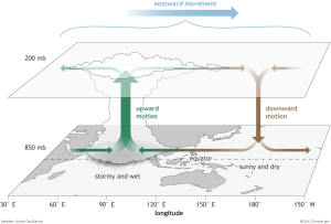
Figure 11 Details.
The surface and upper-atmosphere structure of the MJO for a period when the enhanced convective phase (thunderstorm cloud) is centered across the Indian Ocean and the suppressed convective phase is centered over the west-central Pacific Ocean. (Source: F. Martin, Climate.gov)
The MJO consists of two parts, or phases: one is the enhanced rainfall (or convective) phase and the other is the suppressed rainfall (sunny and dry) phase. These two phases produce opposite changes in clouds and rainfall and this entire dipole (i.e., having two main opposing centers of action) propagates eastward alternating in 40 to 50 days. The MJO can modulate the timing and strength of monsoons, influence tropical cyclone numbers and strength in all ocean basins, and result in jet stream changes that can lead to cold air outbreaks, extreme heat events, and flooding rains over the United States and North America.
Ocean acidification
For more than 200 years, or since the industrial revolution began, the concentration of carbon dioxide (CO2) in the atmosphere has increased due to the burning of fossil fuels and land use change (deforestation, agriculture). During this time, the pH of surface ocean waters has decreased by 0.1 pH units. The pH scale, like the Richter scale, is logarithmic, so this change represents approximately a 30% increase in acidity.
The ocean absorbs about 30% of the CO2 that is released in the atmosphere, and as levels of atmospheric CO2 increase, so do the levels in the ocean. When CO2 is absorbed by seawater, a series of chemical reactions occur resulting in the increased concentration of hydrogen ions. This increase causes the seawater to become more acidic and causes carbonate ions to be relatively less abundant.

Carbonate ions are an important building block of structures such as sea shells and coral skeletons. Decreases in carbonate ions can make building and maintaining shells and other calcium carbonate structures difficult for calcifying organisms such as oysters, clams, sea urchins, corals, and calcareous plankton. The pteropod, or “sea butterfly,” is a tiny sea creature about the size of a small pea. Pteropods are eaten by organisms ranging in size from tiny krill to whales and are a major food source for North Pacific juvenile salmon. When pteropod shells were placed in sea water with pH and carbonate levels projected for the year 2100, the shells slowly dissolved after 45 days. Researchers have already discovered severe levels of pteropod shell dissolution in the Southern Ocean, which encircles Antarctica. Pteropods are small organisms, but imagine the impact if they were to disappear from the marine ecosystem!
Ocean acidification affects the life of non-calcifying organisms, such as Pollock and clown fish. While many species will be harmed by ocean acidification, photosynthetic algae and seagrasses may benefit and increase in numbers from higher CO2 concentrations in the ocean.
Sea Level Rise
Global sea level has been rising over the past century, and the rate has increased in recent decades. In 2014, global sea level was 6.6 cm (2.6 inches) above the 1993 average—the highest annual average in the satellite record (1993-present). The two major causes of global sea level rise are thermal expansion caused by warming of the ocean (since water expands as it warms) and increased melting of land-based ice, such as glaciers and ice sheets. Glaciers and ice sheets, large land-based formations of ice, are melting as global temperatures rise. That meltwater drains into the sea, increasing the ocean’s water volume and global sea level. Melting ice has caused about two-thirds of the rise in sea level to date, one-third from land ice in Greenland and Antarctica and one third from melting ice on mountains.
Ice sheets and glaciers in Greenland and Antarctica melt three ways: from above due to warming air, from the sides as they break off into the sea, and from below due to warming ocean water where the ice extends over the sea. Because of this, the rate of ice melt varies from place to place as conditions change. The Arctic is warming more quickly than the Antarctic, which explains why the ice there is thinning more quickly.
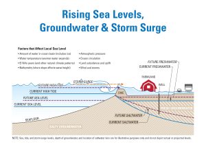
Many glaciers and ice sheets extend into the ocean at their coastal edge, and the floating ice is called an ice shelf. Ice shelves support ice sheets and glaciers by holding the ice on land. But as ocean temperatures increase, warm water laps at the ice shelves, weakening them and causing them to calve glaciers into the sea. This both accelerates ice melting and destabilizes land-based glaciers and ice sheets.
In the future, the melting of ice sheets will dominate sea level rise. Warming has already caused major changes in the ice sheets, continental masses of ice which hold a greater volume of ice than glaciers and ice caps combined. In addition to polar ice, the melting of mountain glaciers, like those in the Andes and Himalayas, has caused an equal amount of sea level rise to date. However, because mountain glaciers include only one percent of all land ice, polar ice will eventually greatly surpass their contributions to global sea-level rise.
One property of water is that warm water takes up more space than cold water. So as the ocean warms from climate change, seawater expands to fill a greater volume and takes up more space. This is called thermal expansion, and it is responsible for one-third of sea level rise to date. When water molecules are heated, they absorb energy. That energy causes the molecules and atoms to move around more and, in the process, take up more space. Thermal expansion is an ongoing contributor to sea level rise as long as ocean water continues to increase in temperature.
This Chapter is compiled from multiple resources including: NASA’s Ocean Motion and Sea Currents, NOAA’s National Centers for Environmental Information, NOAA’s Climate gov., NOAA’s Ocean National Service, Smithsonian Ocean, Intergovernmental Panel on Climate Change, Science, Nature Communications, B. Delorme and Y. Eddebbar: Ocean Climate org., and http://weatherchatroom.forumotion.com/forum.