
5 Chapter 5. Sediment cores, Ice cores and climate change
Sediment cores
History of sediment cores extraction
Deep sea sediment cores provide invaluable information about Earth’s climate in last 200 million years. A long running international collaboration in scientific ocean drilling has transformed human understanding of our planet, addressing fundamental questions about Earth’s dynamic history, processes, and structure. The history of deep-sea coring began in 1940s when Swedish research vessel Albatross used piston coring to recover long and continuous sedimentary cores.
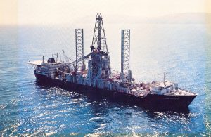
Deep Sea Drilling Program (DSDP) began on June 24, 1966, when the Prime Contract between the National Science Foundation (NSF) and The Regents, University of California was signed. This contract began Phase I of the DSDP, which was based out of Scripps Institution of Oceanography at the University of California, San Diego. Global Marine, Inc. conducted the drilling operations. Glomar Challenger ship was launched on March 23, 1968, from Orange, TX. It sailed down the Sabine River to the Gulf of Mexico, and after a period of testing, DSDP accepted the ship on August 11, 1968.
Phase II consisted of drilling and coring in the Atlantic, Pacific, and Indian Oceans as well as the Mediterranean and Red seas. Technical and scientific reports followed during a Phase II, which ended on August 11, 1972. One of the most important discoveries of the Glomar Challenger was made during Leg 3, when crew drilled different sites along a Atlantic oceanic ridge between South America and Africa. The core samples retrieved provided definitive proof for confirmation of Alfred Wegener’s hypothesis of continental drift and existence of Pangaea supercontinent. The samples gave key evidence to support the
Plate Tectonics Theory
The International Phase of Ocean Drilling (IPOD) began in 1975 with the Federal Republic of Germany, Japan, the United Kingdom, the Soviet Union, and France joining the United States in field work aboard the Glomar Challenger and in subsequent scientific research. The Glomar Challenger docked for the last time with DSDP in November 1983. Parts of the ship, such as its dynamic positioning system, engine telegraph, and thruster console, are stored at the Smithsonian Institution in Washington, DC.
With the advent of larger and more advanced drilling ships, the JOIDES Resolution replaced the Glomar Challenger in January 1985. The new program, called the Ocean Drilling Program (ODP), continued exploration from 1985 to 2003, at which point it was replaced by the Integrated Ocean Drilling Program (IODP).
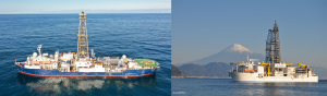
Figure 2 Details.
Left photo: JOIDES Resolution has been used by ODP and IODP for retrieving deep-sea sediment cores since 1985. Right: Japanese research vessel Chikyu has been used by ODP and IODP since 2007. (Source: IODP)
The Integrated Ocean Drilling Program (IODP 2003-2013) built upon the international partnerships and scientific success of the DSDP and ODP by employing multiple drilling platforms financed by the contributions from 26 participating nations. These platforms – a refurbished JOIDES Resolution, the new marine-riser equipped Japanese Deep Sea Drilling Vessel Chikyu, and specialized Mission-Specific-Platforms – were used to reach new areas of the global subsurface during 52 expeditions. Since October 2013, the IODP partners have continued their collaboration via the International Ocean Discovery Program (IODP).
The JOIDES Resolution retrieved core samples in 10 m (30 ft) long cores with a diameter of 10 cm (2.5 in). These cores are currently stored at three IODP repositories in the USA, Germany, and Japan. One half of each core is called the archive half and is preserved for future scientists. The working half of each core is used to provide samples for ongoing scientific research.
Types of sediment coring
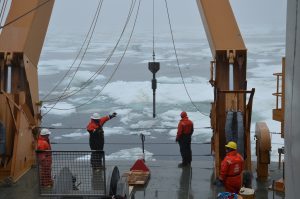
Box Corer
Box Corer is one of the simplest and most commonly used sediment corers. The stainless-steel sampling box can contain a surface sediment block as large as 50cm X 50cm X 75cm with negligible disturbance. The core sample size is controlled by the speed at which the corer is lowered into the ocean bottom. When the bottom is firm, a higher speed is required to obtain a complete sample. A depth pinger or other depth indicator is generally used to determine when the box is completely filled with sediment. Once the core box is filled with sediment, the sample is secured by moving the spade-closing lever arm to lower the cutting edge of the spade into the sediment, until the spade completely covers the bottom of the sediment box. Once the sediment is recovered onboard, the sediment box can be detached from the frame and taken to a laboratory for subsampling and further analysis.
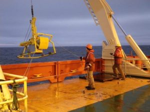
Multi Corers
Multi-corers are designed to recover undisturbed surface sediments from the bottom of the lake or sea. The multi-corer is disposed on a research vessel and is lowered into the sea by a cable. When the multi-corer touches the seafloor the units ballast weight pushes the assembled cores into the seafloor. As a result, each of the tubes contains a unique core with sediment of the seafloor. The sample tubes are sealed with a silicone rubber upper door gasket and a neoprene or carpet lower door seal. Each of the four sample tubes can be removed from MC 400 the coring unit for immediate processing in the laboratory without exposing their contents to the surface environment. Overall sample tube length is 58 cm, with a maximum penetration of 34.5 cm.
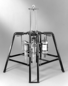
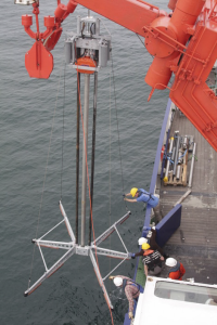
Gravity Corer
Gravity corers are so named because it is gravity that carries the instrument to the seafloor. The corer consists of a metal pipe with a removable lining of plastic tubing typically 1-6 m (3-20 feet) in length. A heavy weight sits atop the pipes. The core is lowered over the side of the ship using a winch and wire rope and is allowed to free fall into the sediments. A core catcher helps trap the sediments in the tubing and the corer is brought back to the surface and aboard the ship.
Vibra corers
Vibracoring is a sediment sampling methodology for retrieving continuous, undisturbed cores. Also referred to as vibrocoring, this mechanical drilling technique is used to collect core samples from unconsolidated, loosely compacted, or semi-lithified materials by driving a tube with a vibrating device. Large, heavy-duty vibracorers can work in water up to 5,000 m deep and can retrieve core samples up to 13 m in length. In coastal shallow water environments where use of heavy equipment is limited by trafficability and ground support on land and high-energy conditions alongshore, cores are shorter, usually about 6 m in length.
Piston corers
The piston corer is a long, heavy tube plunged into the seafloor to extract samples of mud sediment. A piston inside the tube allows scientists to capture the longest possible samples, up to 30 m (90 feet) in length. They are simple and elegant in design, developed in 1947, when Swedish oceanographer Borje Kullenberg made modifications on gravity corer by adding an internal piston that helped researchers gather even longer mud samples. Piston corers, like their cousin the gravity corer, are generally used in areas with soft sediment, such as clay. A gravity corer is just a weighted pipe that is allowed to free fall into the water. Piston corers have a piston mechanism that is triggered when the corer hits the bottom. The piston helps to avoid disturbing or compressing the sediment. A seal on the bottom of the device will retain the sediment sample during retrieval. Special handling equipment is required to safely launch and recover a deep-sea piston coring system.
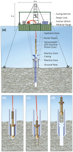
Figure 7 Details.
Hipercoring is the most recent improvement in piston coring. (a). Illustration of coring operations with the coring assembly placed in the hole (b) the corer hammered into sediment (c), and the extraction of coring assembly, including the new core, to the platform while the casing remains in place (d). (Source: Harms et al., 2020)
Climate studies from sediment cores
Oxygen isotope records are preserved in the shells of marine organisms and the proportion of δ18O to δ16O can be revealed by analyzing the chemistry of pristine fossils. The fossils of larger organisms like corals or clams can be especially informative for revealing annual and seasonal temperature variations because these marine animals live for multiple years secreting season growth bands in a similar fashion to tree rings. However, well-preserved clams and corals can be geographically constrained, occurring only in the tropics or in near-shore environments. The most useful for reconstructing ancient seawater temperatures are the microfossils.
The microfossils can speak volumes about the chemistry and temperature of the ocean. The calcium carbonate shells of foraminifera and coccoliths, and the silicon-dioxide shells of radiolarians and diatoms contain both δ18O and δ16O oxygen isotopes. The ratio of these different types of oxygen in the shells can reveal how cold the ocean was and how much ice existed at the time the shell formed. In general, the shells contain more heavy oxygen (δ18O) when ocean waters are cold and ice covers the Earth. Foraminifera occur nearly everywhere in the oceans and have an exquisite fossil record. Thus, the fossil shells of foraminifera can provide a more complete understanding of the ancient ocean’s conditions across all latitudes and at most water depths. By measuring the oxygen isotope ratio in foraminifera, scientists can reconstruct ocean temperatures in past 200 million years.
A large deposit of microfossils can also tell scientists about ocean currents and wind patterns. Ocean plants and animals use the nutrients at the surface of the ocean, die, and then carry the nutrients with them as they sink to the sea floor. In some regions, strong ocean currents sweep nutrients up from the bottom to feed a thriving population. Called upwelling, the phenomenon drives plant and animal populations up until the nutrients are all used, and the microscopic plants and animals die. A small plant called a diatom takes particular advantage of upwelling. Ocean cores hint at patterns of upwelling when one contains a particularly thick layer of microfossils, especially diatoms, from the same time. Since upwelling currents are largely driven by the wind, these patterns also tell scientists something about wind and weather patterns.
Dust in ocean cores can reveal weather and current patterns. Today, great plumes of Saharan dust snake their way across the Atlantic to the American continents. Dust blows into the Pacific from Asia’s vast interior deserts. When the dust shows up in ocean cores, scientists can analyze its chemistry to determine where it came from. By charting the distribution of the dust, scientists can see where the winds were blowing and how strong they were. The dust also gives scientists a glimpse into how dry and dusty the climate may have been at a particular time.
Examples of sediment cores use in climate reconstructions
Recent warming of the Great Lakes water
Instrumental records of surface water temperatures in the Great Lakes indicate warming since 1995. Recent study (Reavie et al., 2016) extracted sediment cores at 10 locations throughout the Great Lakes using research vessels Lake Guardian and Blue Heron, which employed box corers and multiple corers to retrieve sediment. The goal of this research was to study effects of warming water in the Great Lakes examining relative abundance of diatom Cyclotella sensu in the bottom sediments. There is strong evidence that recent atmospheric warming is having an effect on the structure of Great Lakes phytoplankton assemblages. Diatom taxa in the group Cyclotella sensu lato are increasing in relative and absolute abundance in concord with recent, rapid warming. Such a widespread change in the pelagic Great Lakes due to climate change has not been previously observed. The many changes in water column properties that are associated with warming include changes in the duration and extent of open water and ice cover, changes in light and nutrients and changes in stratification and mixing strength.
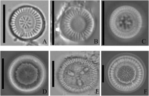
Figure 9 Details.
Light micrographs of diatom Cyclotella sensu lato taxa. (A) Discostella stelligera; (B) Discostella pseudostelligera; (C) Lindavia comensis; (D) Lindavia delicatula; (E) Lindavia ocellata; (F) Lindavia bodanica. Scale bars to left of each taxon indicate 10 μm. (Source: Kireta and Saros, 2019)
Earth’s Climate in Cenozoic Era
Cenozoic Era began 66 million years ago, after an asteroid hit northern Yucatan peninsula and created large Chicxulub crater. Westerhold et al. (2020) used 14 deep-sea cores retrieved by DSDP and ODP cruises using piston coring method. Composite record of Cenozoic climate was derived from stable oxygen (δ18O) and carbon (δ13C) isotopes derived from deep-sea benthic foraminifer genera Cibicidoides and Nuttallides to minimize systematic interspecies isotopic offsets. The accuracy of their chronology ranges from ±100 thousand years (kyr) for the Paleocene and Eocene, ±50 kyr for the Oligocene to middle Miocene, and ±10 kyr for the late Miocene to Pleistocene.
Four distinctive climate states emerge as separate blocks of time designated as the Hothouse, Warmhouse, Coolhouse, and Icehouse states. Warmhouse and Hothouse states prevailed from beginning of Cenozoic Era to the Eocene-Oligocene Transition (EOT), about 34 million years ago. During the Warmhouse, (66 – 56 million years ago, and 47 – 34 million years ago) global temperatures were more than 5°C warmer than they are today. The Hothouse operated between the Paleocene-Eocene Thermal Maximum (PETM) and Eocene Climate Optimum (ECO, 56 – 47 million years ago), when temperatures were more than 10°C warmer than they are today. At the EOT the Warmhouse transitioned into the Coolhouse state, marked by a stepwise, massive drop in temperature and a major increase in continental ice volume with large ice sheets appearing in Antarctica. The Coolhouse state spans from 34 million years ago (EOT) to 3.3 million years ago (mid-Pliocene M2 glacial), and is divided in warmer (34-13.9 Ma), when temperatures were 2-3oC warmer than today, and cooler (13.9-3.3 Ma) periods, with temperatures similar to modern temperatures. The Icehouse climate state, driven by the appearance of waxing and waning ice sheets in the Northern Hemisphere, was fully established by the Pliocene-Pleistocene transition with Marine Isotope Stage M2 at 3.3 million years ago being a possible forerunner. The coldest Icehouse temperatures were about 4oC cooler than modern temperatures. Westerhold et al. (2020) conclude that that climate dynamics during the Warmhouse and Hothouse Cenozoic states are more predictable than those of the Coolhouse and Icehouse states and mostly related to Milankovitch orbital cycles.
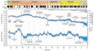
Figure 10 Details.
Cenozoic Global Reference benthic foraminifer carbon and oxygen Isotope Dataset (CENOGRID) from ocean drilling core sites spanning the past 66 million years. (Source: Westerhold et al., 2020)
Ice cores and their use in climate studies
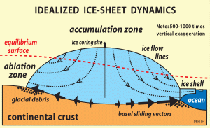
Throughout each year, layers of snow fall over the ice sheets in Greenland and Antarctica. Each layer of snow is different in chemistry and texture, summer snow differing from winter snow. Summer brings 24 hours of sunlight to the polar regions, and the top layer of the snow changes in texture—not melting exactly, but changing enough to be different from the snow it covers. The season turns cold and dark again, and more snow falls, forming the next layers of snow. Each layer gives scientists a treasure of information about the climate each year. Like marine sediment cores, an ice core provides a vertical timeline of past climates stored in ice sheets and mountain glaciers.
The ice cores can provide an annual record of temperature, precipitation, atmospheric composition, volcanic activity, and wind patterns. In a general sense, the thickness of each annual layer tells how much snow accumulated at that location during the year. Differences in cores taken from the same area can reveal local wind patterns by showing where the snow drifted. More importantly, the make-up of the snow itself can tell scientists about past temperatures. As with marine fossils, the ratio of oxygen isotopes in the snow reveals temperature, though in this case, the ratio tells how cold the air was at the time the snow fell. In snow, colder temperatures result in higher concentrations of light oxygen isotope.
When snow forms, it crystallizes around tiny particles in the atmosphere, which fall to the ground with the snow. The type and amount of trapped particles, such as dust, volcanic ash, smoke, or pollen, tell scientists about the climate and environmental conditions when the snow formed. As the snow settles on the ice, air fills the space between the ice crystals. When the snow gets packed down by subsequent layers, the space between the crystals is eventually sealed off, trapping a small sample of the atmosphere in newly formed ice.
These bubbles tell scientists what gases were in the atmosphere and based on the bubble’s location in the ice core, what the climate was at the time it was sealed. The chemical makeup of the air that has been trapped (oxygen, carbon dioxide, and nitrogen) reveals its composition at the time it was buried in the ice. From these measurements, past temperatures are calculated using empirical data and calibrations with modern atmosphere. The temperature record recovered from ice cores goes back about 800,000 years from glaciers that have persisted on landmasses like Greenland and Antarctica.
The most common method for measuring temperatures of ancient Earth uses naturally occurring isotopes. Isotopes are atoms of the same element that are heavier or lighter depending on how many neutrons are in their nuclei. Molecules of water, composed of one hydrogen atom and two oxygen atoms, can have different weights depending on what isotopes of hydrogen and oxygen are bonded together. The two most common isotopes of oxygen in nature are oxygen-16 (16O – 8 neutrons) and oxygen-18 (18O – 10 neutrons).
When the Earth cools down, the lighter isotope 16O is locked away in the ice of high latitude glaciers due to evaporative processes, leaving behind relatively more 18O in the oceans. During warm global climates, melted ice returns 16O-rich waters to the oceans. So the proportion of 18O to 16O in the ocean reflects the Earth’s climate even if we can’t see the ice. Earth Scientists recognize this oxygen isotope pattern between glaciated and ice-free climates, referring to it as the “ice volume effect”, and have since used it to reconstruct ancient Earth climates.
Finally, anything that settles on the ice tends to remain fixed in the layer it landed on. Of particular interest are wind-blown dust and volcanic ash. As with dust found in sea sediments, dust in ice can be analyzed chemically to find out where it came from. The amount and location of dust tells scientists about wind patterns and strength at the time the particles were deposited. Volcanic ash can also indicate wind patterns. Additionally, volcanoes pump sulfates into the atmosphere, and these tiny particles also end up in the ice cores. This evidence is important because volcanic activity can contribute to climate change, and the ash layers can often be dated to help calibrate the timeline in the layers of ice.
Ice sheets have one particularly special property. They allow us to go back in time and to sample accumulation, air temperature and air chemistry from another time. Ice core records allow us to generate continuous reconstructions of past climate, going back at least 800,000 years. By looking at past concentrations of greenhouse gasses in layers in ice cores, scientists can calculate how modern amounts of carbon dioxide and methane compare to those of the past, and, essentially, compare past concentrations of greenhouse gasses to temperature.
Drilling ice cores
The large Greenland and Antarctic ice sheets have huge, high plateaus where snow accumulates in an ordered fashion. Slow ice flow at the center of these ice sheets means that the stratigraphy of the snow and ice is preserved. Drilling a vertical hole through this ice involves a serious effort involving many scientists and technicians, and usually involves a static field camp for a prolonged period of time.
Shallow ice cores (100-200 m long) are easier to collect and can cover up to a few hundred years of accumulation, depending on accumulation rates. Deeper cores require more equipment, and the borehole must be filled with drill fluid to keep it open. The drill fluid used is normally a petroleum-derived liquid like kerosene. It must have a suitable freezing point and viscosity. Collecting the deepest ice cores (up to 3000 m) requires a (semi) permanent scientific camp and a long, multi-year campaign.
History of ice cores
The first ice cores were obtained in 1950s by three separate international research teams:
- the Norwegian–British–Swedish Antarctic Expedition on the Queen Maud Land – now Dronning Maud Land – coast;
- the Juneau Ice Field Research Project in Alaska, and
- the Expeditions Polaires Françaises in central Greenland
These ice cores drilled in the early fifties were about 100 m deep, with generally low quality of ice recovery preventing detailed analytical studies and one can mark the 1957–1958 International Geophysical Year (IGY) as the starting point of ice core research. One of the IGY’s priorities was deep core drilling into polar ice sheets for scientific purposes.
Five nations were particularly active in the early period of deep drilling projects in polar regions – the sixties and seventies – the USA, the Soviet Union, Denmark, Switzerland and France. Cold Regions Research and Engineering Laboratory (CRREL) is the principal US institution involved in ice cores extraction. The drilling operation in Camp Century in northwestern Greenland culminated in the fall of 1960, when it took a strenuous six-year field effort to recover the first ever continuous ice core to the bedrock depth, 1388 m long.
Willi Dansgaard was a pioneer in the establishment of the close link between the isotopic composition of polar snow (δ18O and δD) and the temperature at the precipitation site. Soviet and Russian activities started in 1955 and culminated in the recovery of the deepest core ever obtained, reaching a depth of 3623 m in a project joined in the eighties by French teams and later by US teams. This Vostok drilling was recently extended down to the interface with Lake Vostok at a depth of 3769 m in February 2012. In the eighties the Vostok ice core was the first ice core to cover a full glacial–interglacial cycle. Two other nations, Australia and Canada, started drilling in Polar Regions in the sixties and seventies.
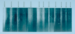
Storing the ice cores
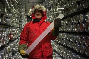
After drilling, measuring and logging an ice core, researchers store the cores in bags or netting in cylindrical tubes. Then they pack the tubes into cardboard boxes or protective waterproof hard cases and transport the cores by sled, plane, boat and truck to storage facilities.
Once the ice cores reach storage facilities, scientists digitally record the ice cores’ characteristics—such as the presence of volcanic ash or the appearance of bubbles in the ice—in a controlled cold laboratory. The U.S. National Ice Core Laboratory (NICL), in Lakewood, Colorado, is the U.S. storage facility, which archives ice cores from all over the world. NICL’s main archive freezer is 55,000 cubic feet in size and is held at a temperature of -36°C.
When a shipment of new ice arrives, the insulated boxes carrying the cores are quickly unloaded into the main archive freezer. Once the new ice has come to thermal equilibrium with its new surroundings, it is carefully unpacked, organized, racked and inspected. After racking, the tubes are checked into NICL’s inventory system. NICL’s storage facility also acts as a library: when scientists want to study a certain ice core from a particular region, they can apply to have a portion of the ice core sent to them for their studies.
Formation of glacier ice
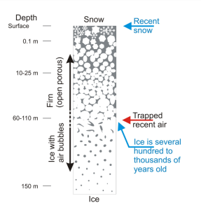
Glaciers begin to form when snow remains in the same area year-round, where enough snow accumulates to transform into ice. Each year, new layers of snow bury and compress the previous layers. This compression forces the snow to re-crystallize, forming grains similar in size and shape to grains of sugar. Gradually the grains grow larger and the air pockets between the grains get smaller, causing the snow to slowly compact and increase in density. After about two winters, the snow turns into firn—an intermediate state between snow and glacier ice. At this point, it is about two-thirds as dense as water. Over time, larger ice crystals become so compressed that any air pockets between them are very tiny. In very old glacier ice, crystals can reach several inches in length. For most glaciers, this process takes more than a hundred years.
Trapping the air in glacier ice
In the firn zone, the air can move relatively freely and therefore exchanges with the atmospheric air. Air bubbles in glacier ice don’t completely close and become isolated from the atmosphere until they are buried by 50-100 meters of snow and ice. The whole process, from snow being compressed into more dense firn and eventually into glacier ice takes anywhere from a few decades in places where snow accumulates quickly (Southern Greenland) to a few thousand years in places with very little snowfall (East Antarctic). That means there is a bit of uncertainty around the exact age of the samples of atmospheric gas contained in the bubbles. The age of the gas in an occluded air bubble is less than the age of the surrounding ice. This age difference (the so-called Δ age) depends on temperature and the amount of snowfall. When interpreting ice core measurements performed on the ice itself together with measurements on the gas in the bubbles, knowledge of Δ age is important. Dedicated firn densification models, based on empirical studies of present-day Greenland and Antarctic conditions, are used to calculate Δ age. These models use information about how the transformation from snow to ice takes place.
Dust trapped in ice cores can change composition of air trapped in bubbles. For instance, since the Greenland Ice Sheet is in the Northern Hemisphere with most of the exposed land on Earth, the ice there contains high amounts of dust. Minerals in that dust do interact with gases preserved in the icy air bubbles, so much so that carbon dioxide records from Greenland ice cores are very difficult to develop. Antarctica preserves much cleaner, clearer gas records because it is very isolated from any of the few Southern Hemisphere land masses, and thus isolated from dust sources.
Layers in glacial ice
Ice cores preserve annual layers, making it simple to date the ice. Seasonal differences in the snow properties create layers – just like rings in trees. Unfortunately, annual layers become harder to see deeper in the ice core. Other ways of dating ice cores include geochemisty, layers of ash (tephra), electrical conductivity, and using numerical flow models to understand age-depth relationships.
Although radiometric dating of ice cores has been difficult, Uranium has been used to date the Dome C ice core from Antarctica. Dust is present in ice cores, and it contains Uranium. The decay of 238U to 234U from dust in the ice matrix can be used to provide an additional core chronology.
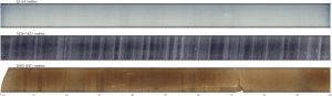
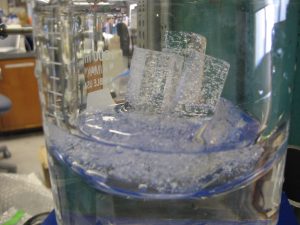
Figure 15 Details.
Relatively young and shallow snow is packed into coarse and granular crystals called firn (top: 53 meters deep). Older and deeper ice has seasonal layers (middle: 1,836 meters). At the bottom of a core (lower: 3,050 meters), rocks, sand, and silt discolor the ice. (Source: U.S. National Ice Core Laboratory)
Information from ice cores
Accumulation rate
The thickness of the annual layers in ice cores can be used to derive a precipitation rate. Past precipitation rates are an important palaeoenvironmental indicator, often correlated to climate change, and it’s an essential parameter for many past climate studies or numerical glacier simulations.
Melt layers
Melt layers are related to summer temperatures. More melt layers indicate warmer summer air temperatures. Melt layers are formed when the surface snow melts, releasing water to percolate down through the snow pack. They form bubble-free ice layers, visible in the ice core. The distribution of melt layers through time is a function of the past climate, and has been used, for example, to show increased melting in the Twentieth Century around the NE Antarctic Peninsula.
Past air temperatures
It is possible to discern past air temperatures from ice cores. This can be related directly to concentrations of carbon dioxide, methane and other greenhouse gasses preserved in the ice. Snow precipitation over Antarctica is made mostly of H216O molecules (99.7%). There are also rarer stable isotopes: H218O (0.2%) and HD16O (0.03%) (D is Deuterium, or 2H). Isotopic concentrations are expressed in per mil δ units (δD and δ18O) with respect to Vienna Standard Mean Ocean Water (V-SMOW). Past precipitation can be used to reconstruct past palaeoclimatic temperatures. δD and δ18O is related to surface temperature at middle and high latitudes.
Snow falls over Antarctica and is slowly converted to ice. Stable isotopes of oxygen (Oxygen [16O, 18O] and hydrogen [D/H]) are trapped in the ice in ice cores. The stable isotopes are measured in ice with a mass spectrometer. Measuring changing concentrations of δD and δ18O through time in layers through an ice core provides a detailed record of temperature change, going back hundreds of thousands of years.
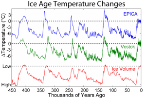
Figure 16 Details.
The changes in ice temperature during the last several glacial-interglacial cycles and comparison to changes in global ice volume. The local temperature changes are from two sites in Antarctica and are derived from deuterium (D) isotopic measurements. The bottom plot shows global ice volume derived from δ18O measurements on marine microfossils. (Source: AntarcticGlaciers.org)
Past gasses in the air
The most important property of ice cores is that they are a direct archive of past atmospheric gasses. The offset between the age of the air and the age of the ice is accounted for with well-understood models of firn densification and gas trapping. The air bubbles are extracted by melting (Fig. 17), crushing or grating the ice in a vacuum. This method provides detailed records of carbon dioxide, methane and nitrous oxide going back almost 800,000 years. Ice core records globally agree on these levels, and they match instrumental measurements from the 1950s onwards, confirming their reliability. Carbon dioxide measurements from older ice in Greenland is less reliable, as meltwater layers have elevated carbon dioxide. Older records of carbon dioxide are therefore best taken from Antarctic ice cores.
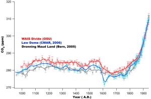
Ahn et al. (2012) report a decadally resolved record of atmospheric CO2 concentration for the last 1000 years, obtained from the West Antarctic Ice Sheet (WAIS) Divide shallow ice core. The most prominent feature of the pre-industrial period is a rapid, about 7 ppm decrease of CO2 in a span of about 20–50 years at about 1600 A.D. This observation confirms the timing of an abrupt atmospheric CO2 decrease of about 10 ppm observed for that time period in the Law Dome ice core CO2 records. Atmospheric CO2 variations over the time period 1000–1800 A.D. are statistically correlated with northern hemispheric climate and tropical Indo-Pacific sea surface temperature. Those records share common trends of CO2 change on centennial to multicentennial time scales, and clearly show that atmospheric CO2 has been increasing above preindustrial levels since about 1850 A.D.
Other major gases trapped in ice cores (O2, N2 and Ar) are also interesting. The stable isotope concentration (δ18O) in ice core records mirrors that of the ocean. Oceanic δ18O is related to global ice volume. Variations of δ18O in O2 in ice core gasses are constant globally, making it a useful chronostratigraphic marker.
Other ice-core uses
In Greenland, volcanic ash layers are preserved in ice cores. The tephra ejected in each volcanic eruption has a unique geochemical signature, and large eruptions projecting tephra high into the atmosphere result in a very wide distribution of ash. These tephra layers are therefore independent marker horizons. Geochemically identical tephra in two different ice cores indicate a time-synchronous event. They both relate to a single volcanic eruption. Tephra is essential for correlating between ice cores, peat bogs, marine sediment cores, varves in lake sediments, etc.
Mineral dust accumulates in ice cores, and changing concentrations of dust and the source of the dust can be used to estimate changes in atmospheric circulation. The two EPICA ice cores (European Project for Ice Coring in Antarctica) contain a mineral dust flux record, showing dust emission changes from the dust source in Patagonia. Changes in the dust emission are related to environmental changes in Patagonia.
This Chapter is compilation from the following sources: International Ocean Discovery Program; Woods Hole Oceanographic Institution; AntarcticGlaciers.org, NASA’s Global Climate Change, NOAA’s National Centers for environmental information, British Antarctic Survey, J. Aagaard, 2015. Measurements of total air content of ice from EUROCORE, Greenland, MS Thesis, Centre for Ice and Climate Niels Bohr Institute, Faculty of Science, University of Copenhagen, Snowball Earth at http://www.snowballearth.org/overview.html, Workshop at NICL Ice Core Repository, Denver, CO, May 2016.