
4 Chapter 4. Paleoclimate studies
Thermometers have only been in widespread use since around 1850. Thus, the instrumental record for earlier times is quite poor and full of gaps. Essentially nothing is available in the way of quantitative measurements of weather conditions for the time before 1800 A.D. To reconstruct climate change, therefore, we need to use indirect indicators. One source of information is historical records: art, logs, dairies, lists on when the wine harvest began, reports on when the ice first broke up in a northern river, or when the cherry trees first blossomed. In some cases, such reports go back hundreds of years, although rarely in unbroken sequence.
Art and paleoclimate
To what extent can paintings or other artworks created during past several centuries be regarded as accurate and reliable guides to atmospheric and weather conditions current at the time? Some recent studies have suggested that art may have a role to help us reconstruct past climates. The reliability of these broad inferences about climate is strengthened where the paintings are prolific, internally consistent and spread over a considerable time. While some of the depictions may be imaginary, symbolic, spiritual and so on, it would seem to be most likely that some and perhaps many of them represented objective reality at the time they were painted, especially where the depictions are supported by other archaeological evidence. Art depictions of glaciers in the mid-19th century provide a useful benchmark against which more recent glacial retreats can be measured. High precision 18th century paintings have been used to identify water levels in Venice in the period before records were kept, and studies of sunsets in a wide range of artworks seem to have provided us with surprisingly accurate indicators of the atmospheric effects of volcanic activity.
Glaciers were expanding and growing larger during Little Ice Age in Europe, but by the mid-19th century many glaciers began to retreat. The effect of warming the climate and disappearance of glaciers can be demonstrated by comparing paintings, engravings or drawings created at that time with more recent photographs of the same scene. The contrast today in the 21st century is particularly dramatic. A comparison of an 1806 glacier sketch with two more recent photographs suggests that the glacier has retreated two kilometers in that period (Figure 1.)

Figure 1 Details.
View of the Mer de Glace, Chamonix, France: Left – sketch by J.M.W. Turner 1806; Middle – photograph by J. Ruskin, 1854; Right – photograph by Emma Stibbon, 2018 (Source: P. McCouat, 2015)
Paleoclimatologists (climatologists who study past or paleo climates) use the term “proxy” to describe a way that climate change is recorded in nature, within geological materials such as ocean or lake sediments, tree-rings, coral growth-bands, ice-cores, and cave deposits. For a proxy to be useful it must first be established that the proxy (i.e. tree-ring width, stable isotope composition of ice, sediment composition) is in fact sensitive to changes in temperature or some other environmental parameter. This phase of research is known as calibration of the proxy.
Tree rings and paleoclimate
The study of the annual growth of trees and the consequent assembling of long, continuous chronologies for use in dating wood is called dendrochronology. The study of the relationships between annual tree growth and climate is called dendroclimatology. Dendroclimatology offers a high resolution (annual) form of palaeoclimate reconstruction for most of the Holocene.
The annual growth of a tree is the net result of many complex and interrelated biochemical processes. Growth may be affected by many aspects of the microclimate: sunshine, precipitation, temperature, wind speed and humidity. Besides these, there are other non-climatic factors that may exert an influence, such as competition, defoliators and soil nutrient characteristics.
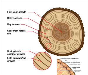
Not all trees are suitable for dendroclimatology. Many trees in tropical areas where growth is not seasonal do not reliably reflect varying conditions and are unsuitable as proxy indicators of palaeoclimates. A cross section of most temperate forest tree trunks will reveal an alternation of lighter and darker bands, each of which is usually continuous around the tree circumference. These are seasonal growth increments produced by meristematic tissues in the cambium of the tree. Each seasonal increment consists of a couplet of earlywood — a light growth band from the early part of the growing season, and denser latewood — a dark band produced towards the end of the growing season, and collectively they make up the tree ring. The latewood of a tree ring is much denser than the earlywood and interannual variations contain a strong climatic signal. The mean width of the tree ring is a function of many variables, including the tree species, tree age, soil nutrient availability, and a whole host of climatic factors. The problem facing the dendroclimatologist is to extract whatever climatic signal is available in the tree-ring data from the remaining background “noise”.
Whenever tree growth is limited directly or indirectly by some climate variable, and that limitation can be quantified and dated, dendroclimatology can be used to reconstruct some information about past environmental conditions. Only for trees growing near the extremities of their ecological amplitude, where they may be subject to considerable climatic stresses, is it likely that climate will be a limiting factor. Commonly two types of climatic stress are recognized, moisture stress and temperature stress. Trees growing in semi-arid regions are frequently limited by the availability of water, and dendroclimatic indicators primarily reflect this variable. Trees growing near the latitudinal or altitudinal treeline are mainly under growth limitations imposed by temperature; hence dendroclimatic indicators in such trees contain strong temperature signals.
Several assumptions underlie the production of quantitative dendroclimatic reconstructions. First, the physical and biological processes which link today’s environment with today’s variations in tree growth must have been in operation in the past. This is the principle of uniformitarianism. Second, the climate conditions which produce anomalies in tree-growth patterns in the past must have their analogue during the calibration period. Third, climate is continuous over areas adjacent to the domain of the tree-ring network, enabling the development of a statistical transfer function relating growth in the network to climate variability inside and outside of it. Finally, it is assumed that the systematic relationship between climate as a limiting factor and the biological response can be approximated as a linear mathematical expression.
Pollen and paleoclimate
Pollen grains are the sperm-carrying reproductive bodies of seed plants like conifers, cycads, and flowering plants. Each of these grains has its very own unique shape depending on what plant it comes from, and their walls are made of a substance known as sporopollenin, which is very chemically stable and strong. The study of pollen is called Palynology.
When pollen grains are washed or blown into bodies of water, their tough outer walls allow them to be preserved in sediment layers in the bottoms of ponds, lakes, or oceans. Because of their unique shapes, palynologists can then take a core sample of the sediment layers and determine what kinds of plants were growing at the time the sediment was deposited. Knowing what types of plants were growing in the area allows the palynologists to make inferences about the climate at that time by using knowledge about modern and historical distributions of plants in relation to climate.
Once they take a core sample, the palynologists isolate the pollen and spores from the sediments and rocks using both chemical and physical means. The grains are very small, typically between 10 and 200 microns, which requires mounting them on microscope slides for examination. The scientists then count and identify the grains using a compound microscope and generate diagrams of the type and abundance of pollen in their samples.
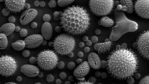
Figure 3 Details.
Scanning Electron Microscopic image of pollen grains from sunflower, morning glory, prairie hollyhock, oriental lily, evening primrose, and castor bean. (Source: NASA)
By analyzing pollen from well-dated sediment cores, palynologists can obtain records of changes in vegetation going back hundreds of thousands, and even millions of years. Not only can pollen records tell us about the past climate, but they can also tell us how we are impacting our climate. Comparing trends in vegetation from the last few thousand years to recent trends in vegetation can also help scientists determine whether human activities have had significant impacts on ecosystems.
Speleothems and paleoclimate
Caves develop in terrains made of carbonate rocks, limestone and dolomite. As water runs through the ground, it picks up minerals, the most common of which is calcium carbonate. When the mineral-rich water drips into caves, it leaves behind solid mineral deposits. The mineral deposits accumulate in the well-known icicle-shaped rock on the ceiling, a stalactite, and in a mound on the floor where the drip lands, a stalagmite.
Geologists refer to the mineral formations in caves as “speleothems.” While the water flows, the speleothems grow in thin, shiny layers. The amount of growth is an indicator of how much ground water dripped into the cave. Little growth might indicate a drought, just as rapid growth could point to heavy precipitation (Figure 6). When the speleothems stop growing, the outside becomes dirty and eroded in places, giving it a dull appearance. A growing speleothem looks smooth and wet.
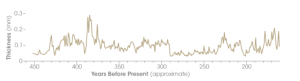
Figure 4 Details.
This graph shows the thickness of annual growth rings for the past 450 years from a stalagmite in Carlsbad Cavern. Thick rings indicate a relatively wet climate, while thin rings indicate a dry climate. (Source: NASA; Graph based on data from Polyak and Asmerom 2001)
Scientists can date the layers in the speleothem by measuring how much uranium, a radioactive element, has decayed. Uranium from the surrounding bedrock seeps into the water and forms a carbonate that becomes part of each layer of the speleothem as it forms. Uranium decays into thorium, which sticks to the clay in the bedrock instead of seeping into ground water and from there into the speleothem. As a result, the newest layers of a growing speleothem typically contain no thorium.
Over time uranium predictably turns into thorium, so scientists can tell how old a layer is by measuring the ratio of uranium to thorium. Once the layers have been dated, scientists can create a rough record of how ground water levels changed over the lifetime of the formation. Because speleothem growth is influenced by geography, ground water chemistry, and other factors, the record from one cave cannot serve as a record of climate change. Scientists must look for similar patterns of growth in speleothems in caves over a broad area to infer that the climate changed.
Recently, scientists have started to use the oxygen isotope ratio to track changes in the amount of rainfall (heavy rain results in more light oxygen) or changes in where the rain came from the ocean or inland sources. In southeast Brazil, for example, winter rain comes from the nearby Atlantic Ocean, but summer rain comes from the Amazon Basin. The two rain sources have quite different oxygen isotope ratios. By examining the oxygen isotopic signatures in the stalactites scientists can track seasonal changes and rainfall patterns. Since caves exist all over the Earth, speleothems have the potential to become a pivotal land-based climate record.
Coral reefs and paleoclimate
Many coral reefs have been around for millions of years, yet they are extremely sensitive to changes in climate conditions. Corals are affected by ocean warming (sometimes bleaching when temperatures rise or fall), by pollution and runoff, and by changes in the pH of seawater, which decreases as more carbon dioxide enters the ocean—a trend known as ocean acidification.
As corals grow, they form skeletons by making calcium carbonate from the ocean waters. The density of these calcium carbonate skeletons changes as the water temperature, light, and nutrient conditions change, giving coral skeletons formed in the summer a different density than those formed in the winter. These seasonal variations in density produce growth rings similar to those in trees or speleothems. Scientists can study these rings and other characteristics to determine the climatic conditions during the seasons in which the coral grew. These growth bands also allow scientists to date coral samples to an exact year and season.
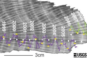
Figure 5 Details.
X-ray image of the annual density bands in corals. Time series of Sr/Ca data are overlain on the x-radiograph to verify that annual bands have been counted correctly. Each Sr/Ca maximum (winter) to maximum (winter) represents an annual temperature cycle. (Source: USGS)
To gather data and information about coral growth bands, scientists use a hollow, diamond-tipped drill bit to gather small core samples from the corals without injuring the animal. Sometimes the banding patterns in these samples are evident by visual inspection alone, but often scientists use x-ray imaging software to get a look at the patterns. The scientists then mark the varying layers by year and season and extract samples from the layers for precise chemical analysis.
Analyzing the composition of trapped oxygen atoms for example, is used to estimate seasonal temperature and rainfall and to build a record of how they have changed through time. Times of environmental stress, including disease outbreaks or bleaching—when a coral animal expels the symbiotic algae that lives within it and gives it its color—can also be identified within the banding. Such markers help scientists determine extreme climate conditions that are harmful to the reef.
By using corals to determine the past climate in the tropical oceans, scientists can also predict future trends in the climate system. The information corals provide about the tropical oceans can be very useful in examining the El Niño Southern Oscillation. El Niño, which is spawned in the Pacific Ocean, greatly affects weather from Asia and Australia to North and South America. By sampling corals in the Pacific, scientists can determine El Niño patterns over the past few hundred years and use that information to improve predictions about future episodes and changes in this natural climate pattern.
Recent climate extremes revealed by proxy data
Last Glacial Maximum (LGM)
Note: Most dates that relate to the end of Pleistocene and early Holocene have B.P. connotation. B.P. refers to Before Present, a time scale used mainly in archaeology and geology to specify when events occurred in the past. Because the “present” time changes, standard practice is to use 1 January 1950 as the commencement date of the age scale, reflecting the origin of radiocarbon dating in the 1950s. So, when you see a reference year 12,000 B.P. that means event actually happened 10,050 years ago (12,000-1950 (BP) = 10,050 years ago). Remember this and always subtract 1950 from dates with B.P references in order to know how long ago such event happened.
During the Last Glacial Maximum (LGM) ice sheets reached their maximum across the world, after a period of global cooling caused by variations in the Earth’s orbit around the sun. There was a massive Laurentide Ice Sheet in North America, a large Eurasian Ice Sheet covering Britain, Ireland and Scandinavia as well as northern Europe, an ice sheet in Antarctica, the Himalaya and Patagonia. Land near the ice sheets that escaped glaciation was cold, with tundra vegetation, frequented by ice-age animals such as mammoth, mastodon, giant elk, reindeer and arctic hare. There were land bridges between Siberia and Alaska and between Britain and Europe, and humans and animals could walk across them. Numerous human artefacts from this time are scattered across the landscape.
The Last Glacial Maximum (LGM) is widely used to refer to the episode when global ice volume last reached its maximum and associated sea levels were at their lowest. However, the boundaries of the interval are ill-defined and the term and acronym have no formal stratigraphical basis. This is despite a previous proposal to define it as a chronozone in the marine records on the basis of oxygen isotopes and sea levels, spanning the interval 23,000-19,000 years ago or 24,000-18,000 years ago and centered on 21,000 years ago. In terrestrial records the LGM is poorly represented since many sequences show a diachronous response to global climate changes during the last glacial cycle. For example, glaciers and ice sheets reached their maximum extents at widely differing times in different places. In fact, most terrestrial records display spatial variation in response to global climate fluctuations, and changes recorded on land are often diachronous, asynchronous or both, leading to difficulties in global correlation. However, variations in the global hydrological system during glacial cycles are recorded by atmospheric dust flux and this provides a signal of terrestrial changes.
Whilst regional dust accumulation is recorded in loess deposits, global dust flux is best recorded in high-resolution polar ice-core records, providing an opportunity to define the LGM on land and establish a clear stratigraphical basis for its definition. On this basis, one option is to define the global LGM as an event between the top (end) of Greenland Interstadial 3 and the base (onset) of Greenland Interstadial 2, spanning the interval 27,540-23,340 years ago (Greenland Stadial 3). This corresponds closely to the peak dust concentration in both the Greenland and Antarctic ice cores and to records of the global sea-level minima. This suggests that this definition includes not just the coldest and driest part of the last glacial cycle but also the peak in global ice volume. The later part of the LGM event is marked by Heinrich Event 2, which reflects the onset of the collapse of the Laurentide Ice Sheet at ~ 24,000 years ago, together with other ice sheets in the North Atlantic region.
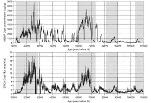
Figure 6 Details.
The ice-core records from Greenland (NGRIP) and Antarctica (EPICA) showing peaks in dust concentration around 23 Ka (LGM or MIS 1) and 70 Ka (MIS4). (Source: Ruth et al., 2007 and Lambert et al., 2012)
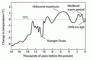
Following the Last Glacial Maximum at the end of Pleistocene and in Holocene, the climate changed several times through abrupt warming phases punctuated by abrupt cooling phases. These events include: Dansgaard–Oeschger events, Heinrich Events, Older Dryas, Bølling-Allerød warm phase, Younger Dryas, Bond Events, Holocene Cooling, Holocene Optimum, Medieval Warm Period, and Little Ice Age.
Dansgaard–Oeschger and Heinrich Events
Climate during the last glacial period was far from stable. Dansgaard-Oeschger and Heinrich events, occurred repeatedly throughout most of this time. Scientists Willi Dansgaard and Hans Oeschger first reported the Dansgaard-Oeschger (D-O) events in Greenland ice cores. Each of the 25 observed D-O events consisted of an abrupt warming to near-interglacial conditions that occurred in a matter of decades and was followed by a gradual cooling.
Related to some of the coldest intervals between D-O events were six distinctive events, Heinrich Events (named after paleoclimatologist Hartmut Heinrich) that are recorded in North Atlantic marine sediments as layers with a large amount of coarse-grained sediments derived from land. These layers, which are continuous across large areas of the North Atlantic, are evidence for both an increase in icebergs discharged from the Laurentide ice sheet in North America and a southward extension of cold, polar waters. Icebergs carry sand-sized grains eroded by ice sheets. When icebergs encounter warmer ocean water, they melt and drop their sediment load onto the seafloor. A southward extension of cold, polar waters allowed icebergs to travel farther before melting. Heinrich events occurred less frequently than D-O events. D-O events repeated every several thousand years on average, while ~10,000 years elapsed between Heinrich events. Neither of the two types of events is strictly periodic, however.
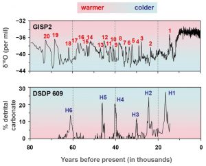
Figure 8 Details.
The δ18O record from the GISP2 ice core in Greenland (top), showing 20 of the 25 observed Dansgaard–Oeschger events during the last glacial period (Grootes et al. 1993). A record of ice-rafted material during Heinrich events (bottom) from a deep-sea core in the North Atlantic (Bond and Lotti 1995).
Near the end of Pleistocene ice sheets released large amounts of freshwater into the North Atlantic. Heinrich events are an extreme example of this, when the Laurentide ice sheet disgorged excessively large amounts of freshwater into the Labrador Sea in the form of icebergs. These freshwater dumps reduced ocean salinity enough to slow deep water formation and the thermohaline circulation. Since the thermohaline circulation plays an important role in transporting heat northward, a slowdown would cause the North Atlantic to cool. Later, as the addition of freshwater decreased, ocean salinity and deep water formation increased and climate conditions recovered. Measurements from deep-sea sediments in the North Atlantic indicate reduction of deep water formation during Heinrich events.
Although the classic interpretation of Heinrich events being produced by internal Laurentide ice-sheet oscillations had some deficiencies, its simplicity permitted it to survive 2 decades. However, recent articles finally shed light on the mystery of how Heinrich events are triggered. Marcott et al. (2011) reported Mg/Ca data from the northwest Atlantic Ocean revealing an AMOC (Atlantic meridional overturning circulation) slowdown accompanied by a large subsurface warming that occurred more than 1,000 years before Heinrich events. The crux, indeed, resided in the subsurface of the ocean. Thanks to recent observations around Antarctica, the poorly understood coupled effects between ocean and ice-sheet dynamics have been revealed to be crucial for understanding past massive iceberg purges. In this way, the observed control that a warming ocean exerts on the ice-streams regime, combined with the confirmed anticipation of an AMOC slowdown and a large subsurface warming, clearly indicates a climatic precursor for Heinrich events. The scenario can thus be summarized as follows (Fig. 11 illustrates the mechanism specifically for Heinrich event 1):
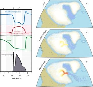
Figure 9 Details.
Schematics of the Heinrich event 1. Left: Time series illustrate the evolution of the main variables involved with the triggering mechanism. A, B, and C indicate critical steps in the Laurentide ice sheet around Heinrich event 1. Right: Warm colors in B and C represent acceleration and thinning in ice streams of the Hudson Bay and Hudson Strait area. (Source: PNAS)
- A change in the mode of oceanic circulation favors a reduction in North Atlantic Deep Water formation and an AMOC slowdown. With reduced convection, the subsurface oceanic layer progressively warms, increasing the rate of basal melting under the Labrador Sea ice shelf.
- Once the depth of crevasses in the ice shelf represents a high proportion of the thinning ice shelf, this latter abruptly collapses. A first very pronounced peak in calving is produced.
- The missing buttressing effect previously exerted by the ice shelf favors a strong ice-stream acceleration, thus transporting inland-ice and detritus into the Atlantic that translate (i) into a sea-level rise of up to 2 m and (ii) into the Heinrich layer observed in marine sediments.
The warm Dansgaard-Oeschger events are then caused by the succeeding re-establishment of the oceanic heat transport strength. Changes from cold climatic conditions to the 10-15°C warmer Greenland temperatures during the Dansgaard-Oeschger events are believed to have occurred within a few decades.
The Oldest Dryas
The complete sequence of late Pleistocene climatic periods are the Oldest Dryas (stadial), the Bölling (interstadial), the Older Dryas (stadial), the Allerød (interstadial), and the Younger Dryas (stadial). The Holocene begins immediately afterward. In some regions the Older Dryas is missing or it is negligible in the evidence. In that case, the initial part of the sequence appears to be Oldest Dryas (cold), Bølling-Allerød (warm), Younger Dryas (cold).
All three Dryas (Oldest, Older, and Younger) are named after a flower (Dryas octopetala) that grows in cold conditions and became common in North America and Europe during those times. Oldest Dryas is a cold episode near the end of Pleistocene that is correlated with the last Heinrich event and occurred between 14,550 and 12,750 years ago. Data derived from isotope variation of nitrogen and argon trapped in Greenland ice cores gives a high-resolution date for the end of the oldest Dryas at the sharp temperature rise of 12,720 years ago.

The Bølling-Allerød interstadial
The Bølling-Allerød interstadial was an abrupt warm and moist interstadial period that occurred during the final stages of the last glacial period. This warm period lasted from 12,750 – 10,750 years ago. It began at the end of the cold Oldest Dryas, and ended abruptly with the onset of the Younger Dryas, a cold period that reduced temperatures back to near-glacial levels within a decade. In some regions, a cold period known as the Older Dryas can be detected in the middle of the Bølling-Allerød interstadial. In these regions the period is divided into the Bølling oscillation, which peaked around 12,550 years ago, and the Allerød oscillation, which peaked closer to 11,050 years ago.
Bølling-Allerød event coincides with or closely follows a meltwater pulse into North Atlantic, when global sea level rose ~16 m, at rates of 26–53 mm/yr. Records obtained from the Gulf of Alaska show abrupt sea-surface warming of about 3 °C (in less than 90 years), matching ice-core records that register this transition as occurring within decades. In recent years research tied the Bølling-Allerød warming to the release of heat from warm waters originating from the deep North Atlantic Ocean, possibly triggered by a strengthening of the Atlantic meridional overturning circulation at the time.
The Older Dryas
The Older Dryas was a cold period between the Bølling and Allerød warmer phases approximately 12,500 to 11,000 years ago. Its age is not well defined, with estimates varying by 400 years, but its duration is agreed to have been around two centuries. The Older Dryas was a variable cold, dry period, observed in climatological evidence in only some regions, depending on latitude. In regions where it is not observed, the Bølling-Allerød is considered a single warm period. Evidence of the Older Dryas is strongest in northern Eurasia.
The Younger Dryas
The Younger Dryas is one of the most well-known examples of abrupt climate change. About 11,000 years ago, Earth’s climate began to shift from a cold glacial world to a warmer interglacial state. Partway through this transition, around 10,950 years ago, temperatures in the Northern Hemisphere suddenly returned to near-glacial conditions. This cold period is called the Younger Dryas. The end of the Younger Dryas, about 9,550 years ago, was particularly abrupt. In Greenland, temperatures rose 10°C (18°F) in a decade.
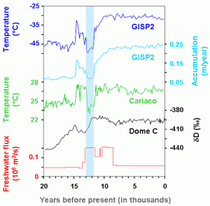
Figure 11 Details.
Climate changes associated with the Younger Dryas, highlighted here by the light blue bar, include (from top to bottom): cooling and decreased snow accumulation in Greenland, cooling in the tropical Cariaco Basin, and warming in Antarctica. Also shown is the flux of meltwater from the Laurentide Ice Sheet down the St. Lawrence River. (Sources: Alley, 2000; Lea et al., 2003; EPICA, 2004; Licciardi et al., 1999).
The Younger Dryas occurred during the transition from the last glacial period into the present interglacial, the Holocene. During this time, the Laurentide Ice Sheet was rapidly melting and adding freshwater to the ocean. Scientists have hypothesized that, just prior to the Younger Dryas, meltwater fluxes were rerouted from the Mississippi River to the St. Lawrence River. Geochemical evidence from ocean sediment cores supports this idea. A more northerly routing of meltwater has a greater impact on the salinity and density of the surface ocean in the North Atlantic, which can cause a slowing of the ocean’s thermohaline circulation and climate changes around the world.
Multiple proxies for the thermohaline circulation indicate that such changes occurred during the Younger Dryas. The record from Dome C in Antarctica supports this explanation. If the thermohaline circulation were to slow, less heat would be transported from the South Atlantic to the North Atlantic. This would cause the South Atlantic to warm and the North Atlantic to cool. Eventually, as the meltwater flux abated, the thermohaline circulation strengthened again and climate recovered.
Bond events
Bond events are North Atlantic ice rafting events that are linked to climate fluctuations in the Holocene, named after Gerard C. Bond, the lead author of the 1997 paper that postulated the theory of cold climate cycles in the Late Pleistocene and Holocene, mainly based on petrologic tracers of drift ice in the North Atlantic. Three indicators found in deep sea cores were used to define the cold events: 1) number of grains with diameters greater than 150 μm; 2) the presence of volcanic glass, mainly from the Iceland or Jan Mayen Island; 3) hematite-stained quartz or Pleomorphic Adeiaoma Gene (PLAG). When IRD peaks as manifested by the three indicators at the sampled locations, it was regarded as the cold events occurred at those locations.
There were nine confirmed cold events during the Holocene, occurring at 11,100 10,300, 9,400, 8,100, 5,900, 4,200, 2,800, 1,400, and 400 years ago. Studies have indicated that the four Bond Events occurring in the early Holocene may be related to freshwater pulses from ice melting in the northern part of the North Atlantic, and the other five Bond Events that occurred during the middle and late Holocene may be related to the decreased solar activity.
Holocene Cooling ~ 8,200 years ago
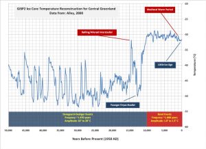
Following the end of the last glacial period about 11,500 years ago, Earth’s climate system began to look and behave more like it does today. The large continental ice sheets shrank, sea level rose, temperatures ameliorated, and monsoons grew in strength. Around 8,200 years ago, however, a surprising event occurred. The 8.2 ka event, was first discovered in the Greenland ice core GISP2, where high-resolution analyses indicate that over two decades temperature cooled about 3.3°C in Greenland. The entire event lasted about 150 years and then temperatures warmed, returning to their previous levels.
The cause of the 8.2 ka event remained a puzzle for some time, but research is converging upon a consistent picture. In the early Holocene, as the large ice sheets of the last glacial period were wasting away, a large proglacial lake (Lake Agassiz) formed south of the Hudson Bay from meltwater. A remnant of the Laurentide ice sheet to the north dammed the proglacial Lake Agassiz. At some point around to 8.2 ka, this dam failed catastrophically, releasing the waters of Lake Agassiz and icebergs from the ice sheet to the Hudson Bay and downstream to the Labrador Sea. Once in the Labrador Sea, these freshwaters changed the density structure of the ocean and slowed deep water formation and the thermohaline circulation.
The Holocene Climate Optimum (HCO)
The Holocene Climate Optimum was a warm period during the interval 7,050 to 3,050 years ago, with a thermal maximum around 6,050 years ago. This period has also been known by many other names, such as Altithermal, Climatic Optimum, Holocene Megathermal, Holocene Optimum, Holocene Maximum, Hypsithermal, and Mid-Holocene Warm Period.
The HCO warm event consisted of increases of up to 4 °C near the North Pole and up to 9 °C in northern central Siberia. Northwestern Europe experienced warming, but there was cooling in Southern Europe. The average temperature change appears to have declined rapidly with latitude. Tropical reefs tend to show temperature increases of less than 1 °C. The tropical ocean surface at the Great Barrier Reef about 5350 years ago was 1 °C warmer and enriched in 18O by 0.5 per mil relative to modern seawater. Other climate changes have been reported, such as significantly wetter conditions in Africa, Australia and Japan. Dry, desert-like conditions were recorded in the Midwestern United States, while Amazon region experienced higher temperatures and drier conditions. It appears that changes in Earth’s orbit (Milankovitch Cycles) caused warmer summers in Northern Hemisphere. This, combined with warmer winters at high latitudes due to reduction of winter sea ice cover caused by more summer melting.
Medieval Warm Period (MWP)
Medieval warm period, also called Medieval Warm Epoch or Little Climatic Optimum, brief climatic interval that is hypothesized to have occurred from approximately 900 to 1300 CE in which relatively warm conditions have prevailed in various parts of the world, though predominantly in the Northern Hemisphere from Greenland eastward through Europe and parts of Asia.
Many studies show that the amount of warming occurring during the MWP varied by season and region. Some provide evidence of relatively warm temperatures during the summer months in several regions, including the North Atlantic, northern Europe, China, and parts of North America, as well as the Andes, Tasmania, and New Zealand. Other studies maintain that the temperature conditions of certain regions, such as the Mediterranean, South America, and other locations in the Southern Hemisphere, were essentially no different from those of the present day.
Only a few studies have attempted to assign a specific value to changes in average global temperatures during the MWP. In 1965 British climatologist Hubert Horace Lamb examined historical records of harvests and precipitation, along with early ice-core and tree-ring data, and concluded that the MWP was probably 1–2 °C (1.8–3.6 °F) warmer than early 20th-century conditions in Europe.
The MWP was a prosperous time in European history. The interval was concurrent with Norse explorations of the New World, the founding of Norse settlements in Iceland and Greenland, and increased agricultural productivity and crop diversity in northern Europe. The pleasant conditions of the MWP allowed the settlements in Iceland and Greenland to prosper and Norse explorers to venture to the coasts of Labrador and Newfoundland to hunt and fish. Extended summers and mild winters lead to plentiful harvests over much of Europe and wheat cultivation and vineyards at latitudes that were further north than today.
Paleoclimatologists have noted that the MWP interval was characterized by an increase in incoming solar radiation paired with a relative absence of volcanic activity. Warmer air temperatures in the North Atlantic region were caused by warmer seawater delivered by the Gulf Stream and other currents.
Little Ice Age (LIA)
The Little Ice Age is the 16th–mid 19th century period of mountain glacier expansion, during which European climate was most strongly impacted. This period begins with a trend towards enhanced glacial conditions in Europe following the warmer conditions of the MWP, and terminates with the dramatic retreat of these glaciers during the 20th century. The LIA was a time of modest cooling of the Northern Hemisphere, with temperatures about 0.3oC cooler than preceding period and 0.8oC colder than late 20th century. The 17th and 19th centuries appear as the coldest centuries within this period. While there is evidence that many other regions outside Europe exhibited periods of cooler conditions, expanded glaciation, and significantly altered climate conditions, the timing and nature of these variations are highly variable from region to region, and the notion of the Little Ice Age as a globally synchronous cold period has all but been dismissed.
The injection of sunlight-reflecting sulfate aerosols by explosive volcanic eruptions may be responsible for some of the cooling of the early and mid-19th century. A prominent example is the 1815 eruption of Tambora in Indonesia that is typically blamed for the year without a summer. While parts of eastern North America and Europe experienced notable cooling, the observation that other regions, including the western US and the Middle East, appear, in fact, to have been warmer than usual is consistent with a hypothesized relationship between volcanic forcing of climate and the response of the North Atlantic Oscillation. The longer-term variations, and in particular cooler temperatures during the 17th century and warmer temperatures during the 18th century were likely to have been related to a concomitant increase in solar output by the Sun by approximately 0.25% following the Maunder Minimum of the 17th century. Finally, changes in the ocean circulation (e.g., the Gulf Stream) of the North Atlantic, and associated impacts on North Atlantic storm tracks, may have emphasized temperature changes in Europe.
This Chapter is compiled from following sources: NASA’s Earth Observatory, Smithsonian National Museum of Natural History, “Art as a barometer of climate changes” by P. McCouat, 2015, Global Climate Change Organization, NOAA National Centers for Environmental Information, Helmholtz Centre for Ocean Research Kiel, Proceedings National Academy of Sciences (PNAS), Encyclopedia Britannica.