34 Errors and Approximations
We begin this next section with the study of numerical methods. We see numerical methods being applied every day in scientific research and engineering, where data approximations and errors are being calculated to lead development in the right direction. In the following subsections of numerical methods we will see some familiar notations such at integrals, differentiation, and various functions from calculus. Much of what we learn in basic math courses such as algebra and calculus lead the way to advanced math concepts like the one we will cover today.
Of the following concepts we will cover, the main job is to calculate the best approximation within range. One of the many benefits to numerical methods and the ability to program the information for computer use. This allows for anyone to input data and quickly run an established macro to output a quick approximation.
With all approximations there is much room for error and not every programmed calculation is always perfect. With this in mind we will begin by covering how to calculate errors and the various methods available, before moving on to numerical integration.
As already mentioned, errors exist in numerical methods because we are making approximations, not spending the time to calculate an exact value for the solution. With any approximation, most likely, the solution is not the exact value. We can also say that the amount the approximation is off by, known as the error, is quantifiable.
Before we can look at approximations we need to understand the different errors and how we calculate them so that when we progress to approximations we are able to calculate the accuracy of the approximation.
We begin with the most straightforward error calculation method, true error.
True Error: Let ![]() be the true value for
be the true value for ![]() at
at ![]() using direct substitution. Let
using direct substitution. Let ![]() be the approximate value for
be the approximate value for ![]() at
at ![]() , using an approximation method. The true error is thus:
, using an approximation method. The true error is thus:
![]()
We will see an example of a true error when we discuss examples of Taylor series. In later subsections we will be introduced to approximations that begin at a point near to our center and we can improve our approximation the more successive calculations we have after the initial approximation. With this kind of approximation environment we usually are not able to calculate the true value at the center point. Therefore we can only calculate the error between successive approximations and through a pattern of approximate errors we can see if the error value is trending down or up which will tell us if the approximations are growing farther away or coming closer together at a center value.
Approximate Error: Let ![]() for some
for some ![]() be the previous value of an approximation and let
be the previous value of an approximation and let ![]() be the current value for the approximation. We calculate the approximate error as
be the current value for the approximation. We calculate the approximate error as
![]()
There is a trend we make out with the errors thus far, each error is calculated as an absolute value. This is done because our starting value for the approximation may be greater or less than the center point we wish to approximate and for that reason we are only concerned with how large the difference is.
We see errors more frequently as percentages in our day to day life. This is why numerical methods teaches us about relative errors. For both true and approximate error we have the following relative error functions.
- True Relative Error: Let
 be the true value for
  at point
  and let
  be the approximate value for
  centered at
  . Then the true relative error can be found as
![]()
- Approximate Relative Error: Let
 be the previous approximate value for
  centered at
  and let
  be the current approximate value for
  centered at
  . Then the approximate relative error can be found as
![]()
Now that we have established how to calculate the errors for out approximations we can introduce the different approximation methods. In the next few subsections we will also be able to understand when different error calculations are applicable and when they are not. Let us begin with the Taylor series approximation and the appropriate method for finding the errors.
28.1 Taylor Series
We have already covered series in a previous section, with this in mind we introduce the Taylor series. The Taylor series is an expansion of a series for the function ![]() about a point
about a point ![]() . We can denote the series as
. We can denote the series as
![]()
We can interpret this notation as follows, beginning with wanting to find the best approximate value for function ![]() at point
at point ![]() . We start the Taylor series by first finding
. We start the Taylor series by first finding ![]() at a close point
at a close point ![]() . As we progress through the series expansion, taking derivatives of
. As we progress through the series expansion, taking derivatives of ![]() at point
at point ![]() and inputting them as the Taylor series requires we are building on our approximation. This means with each calculation we are making our approximation more precise.
and inputting them as the Taylor series requires we are building on our approximation. This means with each calculation we are making our approximation more precise.
At the very end of the Taylor series formula we see an ![]() , this is what is left between the approximation and the true value of a problem. We call
, this is what is left between the approximation and the true value of a problem. We call ![]() the remainder term as it is the total of what remains between the approximation and the true value. The remainder is included in this formula because we began with
the remainder term as it is the total of what remains between the approximation and the true value. The remainder is included in this formula because we began with ![]() not
not ![]() this means that the Taylor series plus the remainder gives the exact value for
this means that the Taylor series plus the remainder gives the exact value for ![]() . To calculate the remainder we have the following equation.
. To calculate the remainder we have the following equation.
![]()
Where ![]() is defined as some point such that
is defined as some point such that ![]() . Since we are approximating the remainder using the
. Since we are approximating the remainder using the ![]() derivative we can compare the remainder to the true error. By comparing the two values with
derivative we can compare the remainder to the true error. By comparing the two values with ![]() we are able to check if our calculations using Taylor series are correct.
we are able to check if our calculations using Taylor series are correct.
Times when the Taylor series and relative error is most useful is when certain functions have a discontinuous point ![]() but we have a desire to calculate the value of
but we have a desire to calculate the value of ![]() at
at ![]() anyways. This is not always the case, in the following example we know we can easily calculate the desired
anyways. This is not always the case, in the following example we know we can easily calculate the desired ![]() but to show the accuracy of the Taylor series we use an example that could also be calculated by substitution.
but to show the accuracy of the Taylor series we use an example that could also be calculated by substitution.
Example:
Given ![]() approximate
approximate ![]() at
at ![]() with
with ![]() through the third derivative.
through the third derivative.
We start by calculating the first three derivatives for ![]() .
.
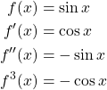
Next we need to calculate each function at ![]()
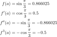
Next we calculate ![]() . Now we can substitute in our found values for the Taylor series format we saw earlier and find the solution rounded to 6 significant figures.
. Now we can substitute in our found values for the Taylor series format we saw earlier and find the solution rounded to 6 significant figures.

Now to find the true error we know that ![]() so we find the true error to be
so we find the true error to be
![]()
Next we must calculate ![]() . Let
. Let ![]() such that
such that ![]() .
.
![]()
Since ![]() we know we have performed our calculations correctly.
we know we have performed our calculations correctly.
This rounds out our discussion on the Taylor series. Next we will cover the series utilized when we are approximating ![]() using
using ![]() , the Maclaurin Series.
, the Maclaurin Series.
28.2 Maclaurin Series
As previously mentioned the Maclaurin series is the Taylor series but for ![]() . This should be very straight forward as we have already been introduced to the formula for the Taylor series as well as the formula for calculating the remainder term of the series. The exact same formulas are utilized for the Maclaurin series. We will jump right into an example.
. This should be very straight forward as we have already been introduced to the formula for the Taylor series as well as the formula for calculating the remainder term of the series. The exact same formulas are utilized for the Maclaurin series. We will jump right into an example.
Example:
Given ![]() approximate
approximate ![]() at
at ![]() with
with ![]() through the fourth derivative [15].
through the fourth derivative [15].
First we begin by finding the derivatives for ![]() through the fourth derivative.
through the fourth derivative.
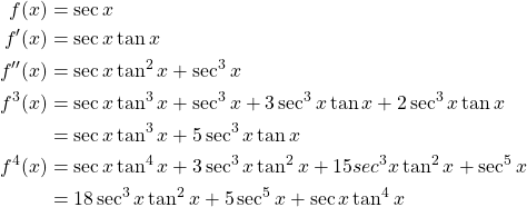
Next we calculate the value for each of the derivatives at ![]() .
.
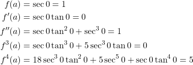
Now we can substitute these found values into the Taylor series formula.

Now to find the true error.
![]()
Next we must calculate ![]() . Let
. Let ![]() such that
such that ![]() .
.
![]()
Since ![]() we know we have performed our calculations correctly.
we know we have performed our calculations correctly.
As we can see from this example everything all the formulas apply the same as in a normal Taylor series, the only difference between Taylor and Maclaurin series is that in Maclaurin series ![]() . The next section of numerical methods we will cover will introduce further measurements for potential inaccuracy in calculations.
. The next section of numerical methods we will cover will introduce further measurements for potential inaccuracy in calculations.
28.3 Analysis
In the real world when we take a measurement we need to take into account that the measurement is not perfect, there is always room for error whether it be human error or computer error. With this in mind numerical methods teaches students exact and approximate analysis. Now this is not the same analysis we learned from our real analysis course where we studied axioms of sets and learned about topology. Here we learn how to account for uncertainty in our calculations.
Exact Uncertainty
We begin with the uncertainty in our measurements for variables of a function. Let ![]() be an arbitrary variable in a function
be an arbitrary variable in a function ![]() . Then
. Then ![]() . This format works for any variable so if we have
. This format works for any variable so if we have ![]() as a variable then
as a variable then ![]() . This formula for a variable, given uncertainty, consists of the mean value denoted by
. This formula for a variable, given uncertainty, consists of the mean value denoted by ![]() and the radius of uncertainty
and the radius of uncertainty ![]() . We define the formula for exact analysis of uncertainty as follows.
. We define the formula for exact analysis of uncertainty as follows.
Definition.
Let ![]() be a function such that
be a function such that ![]() is the mean value for
is the mean value for ![]() and the minimum and maximum values are defined as
and the minimum and maximum values are defined as ![]() respectively. The uncertainty of
respectively. The uncertainty of ![]() can then be defined as follows.
can then be defined as follows.
![]()
In order to fully understand the process of exact analysis we refer to an example.
Example:
Given ![]() , let
, let ![]() and
and ![]() . Find the uncertainty of
. Find the uncertainty of ![]() using exact analysis.
using exact analysis.
First, we can look at the relative uncertainty of ![]() and
and ![]() by the following calculation
by the following calculation

Now to find the uncertainty of ![]() we first need to find
we first need to find ![]() .
.

Next we need to calculate the maximum possible value of ![]() .
.

We must also do the same for the minimum possible value of ![]() .
.

Now we can substitute all these found value in the formula for the uncertainty formula ![]() .
.

Thus we can conclude that the absolute uncertainty is written as ![]() . and we find the relative uncertainty to be
. and we find the relative uncertainty to be
![]()
We see in this example that in order to analyze the uncertainty in our final calculation output from ![]() we need to measure the uncertainty of every variable involved. Once the maximums and minimums have been found we can use this information to measure the uncertainty of the calculations output from
we need to measure the uncertainty of every variable involved. Once the maximums and minimums have been found we can use this information to measure the uncertainty of the calculations output from ![]() .
.
Exact analysis uses maximums and minimums to find the average radius of uncertainty, in the next analysis method we look at what might happen if we attempted to search for the greatest uncertainty.
Approximate Uncertainty
As mentioned previously, approximate uncertainty is another way to measure uncertainty but this time we are going for the greatest possible uncertainty. The approach is slightly different by substituting each variable with its function for possible uncertainty and then expanding the function ![]() before simplifying and substituting in real values. Using the same example as for exact analysis we can see how approximate analysis is applied.
before simplifying and substituting in real values. Using the same example as for exact analysis we can see how approximate analysis is applied.
Example:
Given ![]() , let
, let ![]() and
and ![]() . Find the uncertainty of
. Find the uncertainty of ![]() using approximate analysis.
using approximate analysis.
Firstly, for approximate analysis we need to take the absolute values of the magnitudes for each variable and sum them up as we see here.
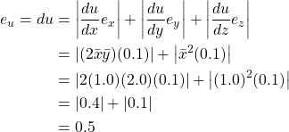
Next we calculate ![]() the same way we did previously, in the exact analysis example.
the same way we did previously, in the exact analysis example.

Thus we have the absolute uncertainty of ![]() as
as ![]() and we can calculate the relative uncertainty the same as the previous example.
and we can calculate the relative uncertainty the same as the previous example.

From this analysis we can also see that the greatest uncertainty of ![]() comes from the uncertainty of
comes from the uncertainty of ![]() since the greatest uncertainty was found to be
since the greatest uncertainty was found to be ![]() where as the greatest uncertainty of
where as the greatest uncertainty of ![]() was
was ![]() .
.
From this previous example showing us the steps of approximate analysis we can see that approximate analysis has a significant benefit. If we needed to find the so called “weakest link” in a calculation we could run an approximate analysis in order to find which variable within the calculation is leading to the a larger uncertainty in the final output. In real life situations this is extremely useful in improving the accuracy of certain measurements within scientific research or engineering.
This concludes our portion of errors and approximations. In the next section we will be reunited with integrals, which we first saw in calculus. This time we will be utilizing integrals in order to approximate an area.
