42 Decision Theory
We have probably exercised some semblance of decision theory throughout our entire life. We have all faced choices where we weighed the pros and cons to choices we are faced with. Decision theory uses models to help measure chance and risk before making a final decision. Businesses use decision theory to figure out how to maximize profit. There are two main categories under decision theory: deterministic and stochastic, we define the two as follows [6].
Definition.
A model where the output is fully determined by the parameter values and the initial conditions.
This means that we can clearly define every option and the parameters are constant, there are no uncontrollable factors at play, there are no risks being weighed or chances we need to take into account. Every parameter in a deterministic model can be determined, there are no random factors [6].
Definition.
A model which possesses some inherent randomness. The same set of parameter values and initial conditions will lead to an ensemble of different outputs.
This model is much more realistic as most situations have a relative amount of random factors at play. Another distinction we need to make in decision theory models is whether the model is to be implemented once as a one time choice or if there are repeated choices. A great example of a repeated decision can be found in gambling. We make the first decision to bet or not, if we win we need to make a decision on if we bet or not again and the choice continues.
When constructing a decision model we also need to take into account if the probability is known or not. If we are thinking of putting a new product into manufacturing we do not know the exact probable demand, we would need to make a rough estimate.
Factors like these are where the risk or chance comes in because we are making a prediction on the potential demand of the product, reflected back through increased revenue. The risk is that if we are wrong about our predicted probability then we may lose much more than if we were to not put the new product into manufacturing. This is why we create decision models, in order to look at all the potential risks and rewards to make the best calculated choice.
Probability
We mentioned probability of an outcome, in order to calculate probability of an event we utilize the following formula [9].
![]()
This is the frequency definition of probability, we use the known frequency of the desired outcome divided by the total possible outcomes to find the percentage for the frequency of the desired outcome occurring. We see this when looking at the probability of rolling a 4 or greater on a die.
Example:
Given a fair 6 sided die, if you roll a 4 or greater you win. The probability of rolling a 4 or greater can be calculated by using the following information. Our total number of outcomes is 6, as there are 6 numbers to a die. The amount of desired outcomes is 3 as the sides with 4,5, or 6 are winning sides. Thus the probability of winning on one roll is as follows.
![]()
Making a choice simply based on probability is easy if the outcome is either you win or you lose. What makes a choice more complex is when we link the weight or probability of different event with different expected value.
Expected Value
Before we can look at the definition of an expected value we need to understand what a payoff is. The payoff is the result of an outcome. In our previous example if rolling a 4 resulted in winning ![]() and rolling a 5 resulted in winning
and rolling a 5 resulted in winning ![]() then our payoff is the dollar amount for each outcome [9].
then our payoff is the dollar amount for each outcome [9].
Definition.
Given the outcomes ![]() each with a payoff
each with a payoff ![]() and corresponding probability
and corresponding probability ![]() with
with
![]()
then the quantity ![]() is the expected value.
is the expected value.
Example:
We have engaged in a business venture assume the probability of success is ![]() ; further assume that if we are successful we make
; further assume that if we are successful we make ![]() , and if we are unsuccessful we lose
, and if we are unsuccessful we lose ![]() . Find the expected value of the business venture [9].
. Find the expected value of the business venture [9].
We know the probability of success is ![]() . We can calculate the probability of failure by subtracting
. We can calculate the probability of failure by subtracting ![]() from the total probability of
from the total probability of ![]() to get the difference, we will denote the probability of failure as
to get the difference, we will denote the probability of failure as ![]() .
.
![]()
We know that the payoff of each possibility so we can calculate the expected value ![]() by the following.
by the following.

So our expected value is ![]()
By calculating the expected value we can see that engaging in the new business venture is the best choice. Now if the expected value came out to a negative amount then we would say that the new venture was not worth it. We can model probability and expected values using a decision tree.
Decision Tree
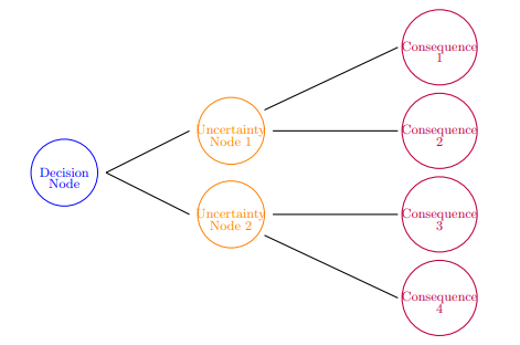
Decision trees are one of the best way to lay out all the possibilities with all the information we have. This allows us to look at all the information and weigh our options. Many times we need to structure our tree beginning with our decision this is where all choices will branch from. The choice branches lead to the uncertainty node, this is where we submit our expected values before expanding branches out for different outcomes that lead to a consequence. For decision trees a consequence does not always have a negative connotation, it simply stands for a result that will occur if we fallow the branch and node map to the end. We can see the basic structure of a decision tree mapped out below.

We now consider an example, utilizing the decision tree
Example:
Assume the following probability distribution of daily demand for bushels of strawberries:
![]()
Further assume that the unit cost is ![]() per bushel, selling price is
per bushel, selling price is ![]() per bushel, and salvage value on unsold units is
per bushel, and salvage value on unsold units is ![]() . We can stock
. We can stock ![]() or
or ![]() units. Assume that the units from any single day cannot be sold on the next day. Build a decision tree and determine how many units should be stocked each day to maximize net profit [9].
units. Assume that the units from any single day cannot be sold on the next day. Build a decision tree and determine how many units should be stocked each day to maximize net profit [9].
Here we need to consider that if one bushel costs ![]() then 2 cost
then 2 cost ![]() and 3 cost
and 3 cost ![]() . Next, we need to consider profit if we sell each bushel for
. Next, we need to consider profit if we sell each bushel for ![]() then to sell one the profit is
then to sell one the profit is ![]() , selling 2 gives us a profit of
, selling 2 gives us a profit of ![]() , and selling 3 would give us
, and selling 3 would give us ![]() . We need to calculate the losses, the salvage value for one bushel is
. We need to calculate the losses, the salvage value for one bushel is ![]() so for one unsold bushel the loss is
so for one unsold bushel the loss is ![]() . If we don’t sell two then the salvage value is
. If we don’t sell two then the salvage value is ![]() with a loss of
with a loss of ![]() , and if we don’t sell three then the salvage value is
, and if we don’t sell three then the salvage value is ![]() with a loss of
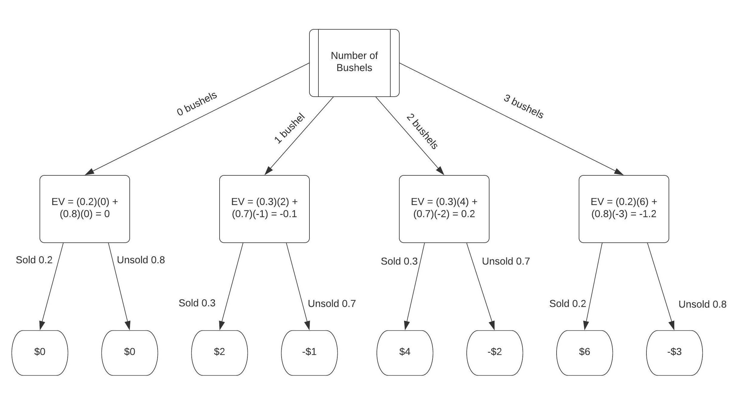
with a loss of ![]() . Now that we have all our information we construct the decision tree as follows
. Now that we have all our information we construct the decision tree as follows

From this diagram we can see that we should stock 2 bushels as it has the greatest expected value of ![]() .
.
This example gives a basic understanding of how we apply the use of a decision tree within math modeling. There are many different ways we can utilize a decision tree but for the basis of decision theory, this is a good introduction. There are more complex trees that build off one another in what we call a sequential decision tree. The tree, in this case, will map out a sequence of outcomes over time. A scenario that involve these more complex trees would be a gambling event. By betting on the outcome of a roulette wheel we can build a sequential tree that we can follow to track the progress of probability and payoffs as we continue through spins.
From one player to multi-player problems, we move from our introduction of decision trees to begin learning about game theory.
