Numerical Integration

Maggie Schildt

35 Numerical Integration

We have seen countless integrals in calculus and have become quite proficient in being able to evaluate integrals. We also saw how Riemann sums could be used to approximate the area under a curve by using mid-points or end points. The next two rules we will cover have a similar intention as Riemann sums the only requirement of these rules is that the integrals must be definite. As well, with using the Trapezoid and Simpson’s rule for approximation there is also the ability to calculate error just as we did previously with series.

29.1 Trapezoid Rule

We begin with the Trapezoid rule. Unlike the Riemann sums which used the sum of the areas of rectangles approximately fitted to the curve of a function to approximate the total area, with Trapezoid rule we include the area of fitted triangles associated with each rectangle. The diagram below gives the best representation to understand this concept.

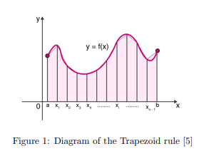
We can see from this diagram that the rectangles we are familiar with from Riemann sums are built upon with triangular ends to better fit the curve. We define the formula for the Trapezoid rule as follows [37].

Theorem: Trapezoid Rule

Given the integral for $f(x)$ from $a$ to $b$ as

$\begin{equation*} \int_{a}^{b}{f(x) \ dx} \end{equation*}$

We can approximate the integral using the Trapezoid rule as follows.

$\begin{equation*} \int_{a}^{b}{f(x) \ dx} \approx T_{n}=\frac{\bigtriangleup x}{2} \left[ f(x_{0})+2f(x_{1})+2f(x_{2})+...+2f(x_{n-1})+f(x_{n})\right] \end{equation*}$

Where $\bigtriangleup x=\frac{b-a}{n}$ for $n\in \mathbb{N}$ intervals and $x_{i}=a+i\bigtriangleup x$ .

The idea behind the Trapezoid rule is that the approximation will become more precise as the number of intervals $n$ grows.

Example:

Evaluate the following integral with $n= 4$ intervals using the trapezoid rule [15].

$\begin{equation*} \int_{0}^{0.5}{(1-x^{2})^{0.5} \ dx} \end{equation*}$

We begin by calculating $\bigtriangleup x$ .

$\begin{equation*} \begin{split} \bigtriangleup x&= \frac{b-a}{n} \\ &=\frac{0.5-0}{4} \\ &=\frac{1}{8} \end{split} \end{equation*}$

Now that we have found $\bigtriangleup x$ , we calculate the values for $f(x)$ at each point starting with $a=0$ as always.

$\begin{equation*} \begin{split} f(0)&=(1-0^{2})^{0.5}=1\\ f(0+0.125)&=(1-(0.125)^{2})^{0.5}=\sqrt{\frac{63}{64}}\\ f(0+2(0.125))&=(1-(0.25)^{2})^{0.5}=\sqrt{\frac{15}{16}}\\ f(0+3(0.125))&=(1-(0.375)^{2})^{0.5}=\sqrt{\frac{55}{64}}\\ f(0+4(0.125))&=(1-(0.5)^{2})^{0.5}=\sqrt{\frac{3}{4}} \end{split} \end{equation*}$

Now substituting our found values into the trapezoid rule function and solve for the approximation.

$\begin{equation*} \begin{split} \int_{0}^{0.5}{(1-x^{2})^{5} \ dx} &\approx \frac{0.125}{2} [ f(a)+2f(a+\bigtriangleup x)+2f(a+2\bigtriangleup x)\\ & +2f(a+3\bigtriangleup x)+2f(a+4\bigtriangleup x)+f(b)]\\ &=(0.0625) \left[ 1+2\sqrt{\frac{63}{64}} +2\sqrt{\frac{15}{16}} +2\sqrt{\frac{55}{64}} + \sqrt{\frac{3}{4}} \right] \\ &=0.4775550114 \end{split} \end{equation*}$

Now that we have established how to evaluate an integral we need to address common ways of calculating the error. First off, looking back at the previous example we were able to evaluate the integral and produce a 10 decimal answer but this is a rounded off answer, in numerical methods we call this truncation. Therefore we need to be able to calculate the error with respect to this truncation. We define the formula for this error as follows.

Truncation Error:

Given an integral for function $f(x)$ from $a$ to $b$ . Using the Trapezoid rule to evaluate the integral we can find the truncation error of the integral as follows [16].

Definition.

$\begin{equation*} E_{TRUN} = -\frac{\bigtriangleup x^{2}(b-a) f''(x)}{12}. \end{equation*}$

Branching out we can utilize this formula in two method, either the maximum error or average error method. We have these two unique methods because within the truncation formula we have a function, $f''(x)$ . We need to be able to find the value for this if we are to complete the evaluation for the error.

Maximum Error

The maximum error is much like the approximate uncertainty we discussed in our section on analysis. We are focused on finding the greatest possible error, with this being said we would want to use the greatest value possible for $f''(x)$ . Let us consider our previous example for $n=4$ .

Example:

Given the following integral for $n=4$ , calculate the maximum error.

$\begin{equation*} \int_{0}^{0.5}{(1-x^{2})^{0.5} \ dx} \end{equation*}$

Let us first find the function for the second derivative of $f(x)$ .

$\begin{equation*} \begin{split} f(x) &= (1-x^{2})^{0.5}=\sqrt{(1-x^{2})}\\ f'(x) &= (0.5)\cdot \frac{1}{\sqrt{(1-x^{2})}} \cdot (-2x) =- \frac{x}{\sqrt{(1-x^{2})}}\\ f''(x) &=- \frac{1}{\sqrt{(1-x^{2})}} + \left[ \frac{-x}{\sqrt{(1-x^{2})^{3}}}\cdot (-0.5)\cdot (-2x)\right] \\ &=- \frac{1}{\sqrt{(1-x^{2})}} - \frac{x^{2}}{\sqrt{(1-x^{2})^{3}}}\\ &=-\frac{1}{\sqrt{(1-x^{2})^{3}}} \end{split} \end{equation*}$

Next, since $f''(x)$ is an increasing function then the value for $f''(x)$ at $b$ is the greatest value produced on the interval $(a,b)$ . Thus we calculate $f''(b)$ for $b=0.5$ to be as follows.

$\begin{equation*} \begin{split} f''(0.5) &= -\frac{1}{\sqrt{(1-(0.5)^{2})^{3}}} \\ &=-\frac{1}{\sqrt{\frac{27}{64}}} \end{split} \end{equation*}$

Now we can substitute our known values into the truncation formula and find the error.

$\begin{equation*} \begin{split} E_{TRUN, max} &= -\frac{\left( 0.125 \right)^{2} \cdot (0.5-0)\cdot \left( -\frac{1}{\sqrt{\frac{27}{64}}} \right) }{12}=\frac{0.0078125}{12}\\ &=0.012028 \end{split} \end{equation*}$

Thus we have found the greatest radius of uncertainty for our approximation of the integral, using the Trapezoid rule. Next, we look at the other method for approximating the error by the average.

Average Error

The average error requires us to calculate the average value for the derivative $f^{N}(x)$ . The equation is given as follows.

$\begin{equation*} f^{N}(x)=\frac{f^{N-1}(b)-f^{N-1}(a)}{b-a} \end{equation*}$

This is the basic formula for finding the average value, when applied to the truncation error formula this means that $N=2$ . Thus we can rewrite the truncation error formula with $f''(x)=\frac{f'(b)-f'(a)}{b-a}$ [16].

$\begin{equation*} E_{TRUN, avg}=-\frac{\bigtriangleup x^{2} (b-a)}{12} \frac{(f'(b)-f'(a)}{b-a} =-\frac{\bigtriangleup x^{2} (f'(b)-f'(a)}{12}. \end{equation*}$

Let us revisit our example again to calculate the average error of the Trapezoid rule for $n=4$ .

Example:

Given the following integral for $n=4$ , calculate the average error.

$\begin{equation*} \int_{0}^{0.5}{(1-x^{2})^{0.5} \ dx} \end{equation*}$

Firstly since $N=2$ then instead of finding the second derivative of the function we only need to find the first. Recall that our average formula utilizes $f^{N-1}(x)$ such that $N-1=2-1=1$ . Thus we find the following derivative.

$\begin{equation*} \begin{split} f(x) &= (1-x^{2})^{0.5}=\sqrt{(1-x^{2})}\\ f'(x) &= (0.5)\cdot \frac{1}{\sqrt{(1-x^{2})}} \cdot (-2x) =- \frac{x}{\sqrt{(1-x^{2})}} \end{split} \end{equation*}$

Now we need to calculate $f'(a)$ and $f'(b)$ . Recall that $a=0$ and $b=0.5$ such that we have the following.

$\begin{equation*} \begin{split} f'(0) &=- \frac{0}{\sqrt{(1-(0)^{2})}}=0\\ f'(0.5) &=- \frac{0.5}{\sqrt{(1-(0.5)^{2})}}= -\frac{0.5}{\sqrt{0.75}} \end{split} \end{equation*}$

Now that we have found all our values we can substitute them into our error formula.

$\begin{equation*} E_{TRUN, avg}=-\frac{ \left( 0.125 \right)^{2} \left[ \left(-\frac{0.5}{\sqrt{0.75}} \right)-(0)\right] }{12} = 0.000752 \end{equation*}$

We should note that the average error is smaller than the maximum error, this is to be expected. This is also very helpful if the average error is, for some reason, larger than the maximum then the calculations need to be checked again. We now move on to an improved Trapezoid rule found in the Simpson’s rule.

29.2 Simpson’s 1/3 Rule

Through countless integration problems throughout mathematics we should have noticed how our approximation of an area is improved by smaller intervals which in turn means we need a greater amount of intervals on $(a,b)$ . This is where Simpson’s $1/3$ rule comes in, this integration method is an improvement upon the Trapezoid rule as it utilized parabolas instead of Trapezoids to best fit the area under a curve. We can see this concept illustrated in the below diagram.

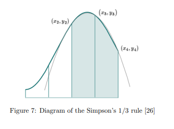
Here we can see that parabolic shapes are built upon the rectangle we know from Riemann sums. With this we can conform to the curve with better accuracy than with the Trapezoid rule’s triangular shapes. We have the formula for the Simpson’s $1/3$ rule as follows.

$\begin{equation*} \begin{split} \int_{a}^{b}{f(x)dx} &= \frac{\bigtriangleup x}{3} [ f(a)+4f(a+\bigtriangleup x) +2f(a+2\bigtriangleup x) + 4f(a+3\bigtriangleup x)\\ &+ 2f(a+4\bigtriangleup x)+...+4f(b-\bigtriangleup x)+f(b)] \end{split} \end{equation*}$

Let us use the same example as before but this time we apply the Simpson’s $1/3$ method.

Example:

Evaluate the following integral with $n= 4$ intervals using the Simpson’s $1/3$ rule [15].

$\begin{equation*} \int_{0}^{0.5}{(1-x^{2})^{0.5} \ dx} \end{equation*}$

For $n=4$ we calculate $\bigtriangleup x$ to be as follows.

$\begin{equation*} \bigtriangleup x=\frac{0.5-0}{4}=0.125 \end{equation*}$

Now we find the values for each $f(x)$ starting with $a=0$ .

$\begin{equation*} \begin{split} f(0)&=\sqrt{(1-(0)^{2}}=1\\ f(0+0.125)=f(0.125)&=\sqrt{(1-(0.125)^{2})}=\sqrt{\frac{63}{64}}\\ f(0+2(0.125))=f(0.25)&=\sqrt{(1-(0.25)^{2})}=\sqrt{\frac{15}{16}}\\ f(0+3(0.125))=f(0.375)&=\sqrt{(1-(0.375)^{2})}=\sqrt{\frac{55}{64}}\\ f(0+4(0.125))=f(0.5)&=\sqrt{(1-(0.5)^{2})}=\sqrt{\frac{3}{4}} \end{split} \end{equation*}$

Now that we have our values we can substitute them into our Simpson’s $1/3$ rule formula.

$\begin{equation*} \begin{split} \int_{0}^{0.5}{(1-x^{2})^{0.5} \ dx} &=\frac{\bigtriangleup x}{3} [f(a)+4f(a+ \bigtriangleup x)+2f(a+2\bigtriangleup x)\\ &+4f(a+3\bigtriangleup x)+f(b)]\\ &= \frac{0.125}{3} \left( 1+4\left( \sqrt{\frac{63}{64}} \right) +2\left( \sqrt{\frac{15}{16}} \right)\\ &+4\left( \sqrt{\frac{55}{64}} \right) +\sqrt{\frac{3}{4}} \right) \\ &=0.4783018038 \end{split} \end{equation*}$

We can compare these values to what we found for this same example using the trapezoid rule, and we will see these are all very close values. What we will really tell us if an improvement has been made is by comparing the errors found for Trapezoid rule versus Simpson’s $1/3$ . We are given the truncation error formula for Simpson’s rule as follows.

$\begin{equation*} E_{TRUN}=-\frac{\bigtriangleup x^{4} (b-a)f^{4}(x)}{180} \end{equation*}$

Using the same example as before we can calculate the maximum truncation error as follows.

Example:

Given the following integral for $n=4$ , calculate the maximum error.

$\begin{equation*} \int_{0}^{0.5}{(1-x^{2})^{0.5} \ dx} \end{equation*}$

Firstly we need to find the fourth derivative for $f(x)$ . We utilize the first two derivatives we found using Trapezoid rule

$\begin{equation*} \begin{split} f(x) &= (1-x^{2})^{0.5}=\sqrt{(1-x^{2})}\\ f'(x) &= (0.5)\cdot \frac{1}{\sqrt{(1-x^{2})}} \cdot (-2x) =- \frac{x}{\sqrt{(1-x^{2})}}\\ f''(x) &=- \frac{1}{\sqrt{(1-x^{2})}} + \left[ \frac{-x}{\sqrt{(1-x^{2})^{3}}}\cdot (-0.5)\cdot (-2x)\right] \\ &=- \frac{1}{\sqrt{(1-x^{2})}} - \frac{x^{2}}{\sqrt{(1-x^{2})^{3}}}\\ &=-\frac{1}{\sqrt{(1-x^{2})^{3}}}\\ f^{3}(x)&=-\frac{1}{\sqrt{1-x^{2})^{5}}} \cdot (-1.5) \cdot (-2x)\\ &=-\frac{3x}{\sqrt{(1-x^{2})^{5}}}\\ f^{4}(x)&=-\frac{3}{\sqrt{(1-x^{2})^{5}}} + \left[ \frac{-3x}{\sqrt{(1-x^{2})^{7}}} \cdot (-2.5) \cdot (-2x) \right] \\ &=-\frac{12x^{2}+3}{\sqrt{(1-x^{2})^{7}}} \end{split} \end{equation*}$

Now we can calculate $f^{4}(x)$ at the maximum $a=0$ since $f^{4}(x)$ is a decreasing function.

$\begin{equation*} f^{4}(0)=-\frac{12(0)^{2}+3}{\sqrt{(1-(0)^{2})^{7}}}=3 \end{equation*}$

Now that we have all of our known values we can calculate the maximum truncation error as follows

$\begin{equation*} E_{TRUN}=-\frac{(0.125)^{4} (0.5-0)(3))}{180}=0.000002 \end{equation*}$

This is a much smaller maximum truncation error than what we found using the Trapezoid rule. Let us now look at the average truncation error and compare to what we found using the Trapezoid rule. Recall that the average is calculated by the following.

$\begin{equation*} f^{N}(x)=\frac{f^{N-1}(b)-f^{N-1}(a)}{b-a} \end{equation*}$

Thus we can calculate the average, given the truncation for Simpson’s $1/3$ requires $f^{4}(x)$ and $4=N$ , as the following.

$\begin{equation*} f^{4}(x)=\frac{f^{3}(b)-f^{3}(a)}{b-a} \end{equation*}$

Which results in the following formula for the average truncation error [16].

$\begin{equation*} E_{TRUN, avg}=-\frac{\bigtriangleup x^{2} (b-a)}{180} \frac{(f^{3}(b)-f^{3}(a)}{b-a} =-\frac{\bigtriangleup x^{2} (f^{3}(b)-f^{3}(a)}{180}. \end{equation*}$

Now we can calculate the average truncation error for our example, this time for Simpson’s $1/3$ rule.

Example:

Given the following integral for $n=4$ , calculate the average error.

$\begin{equation*} \int_{0}^{0.5}{(1-x^{2})^{0.5} \ dx} \end{equation*}$

Firstly we need already found the third derivative for $f(x)$ from the maximum error to be

$\begin{equation*} f^{3}(x)=-\frac{3x}{\sqrt{(1-x^{2})^{5}}} \end{equation*}$

Thus we can calculate the third derivative for $a=0$ and $b=0.5$ as follows.

$\begin{equation*} \begin{split} f^{3}(0)&=-\frac{3(0)}{\sqrt{(1-(0)^{2})^{5}}}=0\\ f^{3}(0.5)&=-\frac{3(0.5)}{\sqrt{(1-(0.5)^{2})^{5}}}=-\frac{16}{9\sqrt{3}} \end{split} \end{equation*}$

Now that we have all our known values we can substitute our values in for the average truncation error formula.

$\begin{equation*} E_{TRUN, avg}=-\frac{(0.125)^{4} (\left( -\frac{16}{9\sqrt{3}} \right) - 0}{180}=0.000045 \end{equation*}$

Again we see that the average truncation error is much smaller for the Simpson’s $1/3$ rule than for the Trapezoid rule. This supports our claim that the Simpson’s $1/3$ rule is an improved version of the Trapezoid rule as we have seen by the simple improvement in error from Trapezoid to Simpson’s $1/3$ rule.

Now so far we have seen integrals with even values of $n$ . What happens if $n$ is odd? This is where Simpson’s $3/8$ rule is utilized.

29.3 Simpson’s 3/8 Rule

The first step of the Simpson’s $3/8$ rule is to separate our integral into two integrals, one with an even amount of intervals and one with the odd remaining intervals. For the integral with an even amount of interval we simply apply the Simpson’s $1/3$ rule. The idea behind the Simpson’s $3/8$ rule is that we initially want an odd integral with $n=3$ intervals which gives us the formula

$\begin{equation*} \begin{split} \int_{a}^{b}{f(x)dx} &= \frac{b-a}{3}\cdot \frac{3}{8} \cdot [ f(a)+3f(a+\bigtriangleup x) +3f(a+2\bigtriangleup x) +\\ &...+3f(b-\bigtriangleup x)+f(b)] \end{split} \end{equation*}$

From here we see that 3 in the numerator and the 3 in the denominator cancel each other out leaving us with the approximation formula as follows.

$\begin{equation*} \int_{a}^{b}{f(x)dx} = \frac{b-a}{8} [ f(a)+3f(a+\bigtriangleup x) +3f(a+2\bigtriangleup x) +...+3f(b-\bigtriangleup x)+f(b)] \end{equation*}$

Utilizing a similar example to the one used to approximate with the Trapezoid and Simpson’s $1/3$ rule we now apply Simpson’s $3/8$ rule.

Example:

Evaluate the following integral using Simpson’s rules with $\bigtriangleup x =0.125$ [15].

$\begin{equation*} \int_{0}^{0.875}{(1-x^{2})^{0.5} \ dx} \end{equation*}$

Firstly we need to make sure $n$ is odd. We calculate $n$ by the following.

$\begin{equation*} n=\frac{0.875-0}{0.125}=7 \end{equation*}$

Thus we need to rewrite the integral into two, making sure to have one integral with $n=3$ intervals. we calculate the interval for each integral by letting $\bigtriangleup x \cdot3 = 0.125\cdot 3=0.375$ thus out first integral has $a=0$ and $b=0.375$ and our second integral has $a=0.375$ and $b=0.875$ .

$\begin{equation*} \int_{0}^{0.875}{(1-x^{2})^{0.5} \ dx} = \int_{0}^{0.375}{(1-x^{2})^{0.5} \ dx}+\int_{0.375}^{0.875}{(1-x^{2})^{0.5} \ dx} \end{equation*}$

Let us evaluate the first integral using Simpson’s $3/8$ rule, we first calculate the values for $f$ starting with $a=0$ .

$\begin{equation*} \begin{split} f(0)&=\sqrt{(1-(0)^{2})}=1\\ f(0+0.125)&=\sqrt{(1-(0.125)^{2})}=\sqrt{\frac{63}{64}}\\ f(0+2(0.125))&=\sqrt{(1-(0.25)^{2})}=\sqrt{\frac{15}{16}}\\ f(0+3(0.125))&=\sqrt{(1-(0.375)^{2})}=\sqrt{\frac{55}{64}}\\ \end{split} \end{equation*}$

Now that we have found all are values, we can substitute them into our Simpson’s $3/8$ formula for evaluating the integral.

$\begin{equation*} \begin{split} \int_{0}^{0.375}{(1-x^{2})^{0.5} \ dx} &= \frac{0.375-0}{8} \left[ 1+3\left( \sqrt{\frac{63}{64}} \right) +3 \left( \sqrt{\frac{15}{16}} \right) +\left( \sqrt{\frac{55}{64}} \right) \right]\\ &=0.366011 \end{split} \end{equation*}$

Now, we need to evaluate the second integral. We begin by finding our values for $f$ starting with $a=0.375$ .

$\begin{equation*} \begin{split} f(0.375)&=\sqrt{(1-(0.375)^{2})}=\sqrt{\frac{55}{64}}\\ f(0.375+0.125)&=\sqrt{(1-(0.5)^{2})}=\sqrt{\frac{3}{4}}\\ f(0.375+2(0.125)&=\sqrt{(1-(0.625)^{2})}=\sqrt{\frac{39}{64}}\\ f(0.375+3(0.125)&=\sqrt{(1-(0.75)^{2})}=\sqrt{\frac{7}{16}}\\ f(0.375+4(0.125)&=\sqrt{(1-(0.875)^{2})}=\sqrt{\frac{15}{64}}\\ \end{split} \end{equation*}$

Now that we have found all our values we can substitute them into our formula for Simpson’s $1/3$ rule for evaluating the integral.

$\begin{equation*} \begin{split} \int_{0.375}^{0.875}{(1-x^{2})^{0.5} \ dx}&=\frac{0.125}{3} \left[ \sqrt{\frac{55}{64}} +4 \sqrt{\frac{3}{4}} +2\sqrt{\frac{39}{64}} + 4\sqrt{\frac{7}{16}} + \sqrt{\frac{15}{64}} \right]\\ &=0.378427 \end{split} \end{equation*}$

Now we need to add the two integrals together to complete our evaluation.

$\begin{equation*} \begin{split} \int_{0}^{0.875}{(1-x^{2})^{0.5} \ dx} &= \int_{0}^{0.375}{(1-x^{2})^{0.5} \ dx}+\int_{0.375}^{0.875}{(1-x^{2})^{0.5} \ dx}\\ &=0.366011+0.378427 = 0.744438 \end{split} \end{equation*}$

Now we should evaluate the average and maximum errors to see if this is a good approximation or not. Just as Trapezoid and Simpson’s $1/3$ rules have their own average and maximum error formulas, the same goes for Simpson’s $3/8$ rule. We begin with the formula for the truncation error of Simpson’s $3/8$ rule.

$\begin{equation*} E_{TRUN}=-\frac{(b-a)^{5} f^{4}(x)}{6480} \end{equation*}$

Beginning with the maximum error we simply find when $f^{4}(x)$ is at its maximum over the interval $(0,0.875)$ . In our example we split our original integral into two and applied the $1/3$ rule to one integral and the $3/8$ rule to the other, accordingly we need to find the maximum error as well.

Example:

We start with the first integral, with $n=3$ intervals, the integral is as follows.

$\begin{equation*} \int_{0}^{0.375}{(1-x^{2})^{0.5} \ dx} \end{equation*}$

In our previous calculation for the maximum truncation using Simpson’s $1/3$ rule we found $f^{4}(x)$ as

$\begin{equation*} f^{4}(x)=-\frac{12x^{2}+3}{\sqrt{(1-x^{2})^{7}}} \end{equation*}$

If we were to graph this function we would see that this is an increasing function which means on the interval $(0,0.375)$ the maximum is when $b=0.375$ . Thus we can calculate the maximum truncation error.

$\begin{equation*} \begin{split} E_{TRUN, max}&=-\frac{(0.375-0)^{5}}{6480} \cdot \frac{-12(0.375)^{2}+3}{\sqrt{(1-(0.375)^{2})^{7}}}\\ &=0.000009 \end{split} \end{equation*}$

Next, we need to calculate the maximum truncation error for the second integral.

$\begin{equation*} \int_{0.375}^{0.875}{(1-x^{2})^{0.5} \ dx} \end{equation*}$

Since this integral qualifies for Simpson’s $1/3$ rule we use the Simpson’s $1/3$ rule maximum truncation error given by the following formula.

$\begin{equation*} E_{TRUN, max}=-\frac{\bigtriangleup x^{4} (b-a)f^{4}(x)}{180} \end{equation*}$

Again since we know that $f^{4}(x)$ is an increasing function the maximum will be reached at $b=0.875$ , thus we have the following calculation.

$\begin{equation*} \begin{split} E_{TRUN, max}&=-\frac{(0.125)^{4} (0.875-0.375)}{180} \cdot \frac{-12(0.875)^{2}+3}{\sqrt{(1-(0.875)^{2})^{7}}}\\ &=0.000673 \end{split} \end{equation*}$

Just as we combined our two approximations for the evaluation of the integral, we do the same for the maximum error. Thus our maximum error for the original integral is as follows.

$\begin{equation*} E_{TRUN, max}=0.000009+0.000673=0.000682 \end{equation*}$

Next we need to calculate the average truncation error. In Simpson’s $1/3$ rule we are introduced to finding the average of $f^{4}(x)$ by the formula

$\begin{equation*} f^{4}(x)=\frac{f^{3}(b) - f^{3}(a)}{b-a}. \end{equation*}$

Keeping the truncation formula for Simpson’s $3/8$ rule as is we can calculate our average truncation error for our example. To calculate the average truncation error, we use the same idea of summing two truncation error calculations as we did in the example previous. This time we apply the average calculations. Firstly we know the formula for the average $f^{4}(x)$ is given as follows.

$\begin{equation*} f^{4}(x)=\frac{f^{3}(b)-f^{3}(a)}{b-a} \end{equation*}$

From here we can simplify the formula for the average truncation error.

$\begin{equation*} \begin{split} E_{TRUN}=-\frac{(b-a)^{5}}{6480} \cdot \frac{f^{3}(b)-f^{3}(a)}{b-a} =-\frac{(b-a)^{4}(f^{3}(b)-f^{3}(a)) }{6480} \end{split} \end{equation*}$

Now let us apply this formula to our example.

Example:

We begin with out first of two integrals.

$\begin{equation*} \int_{0}^{0.375}{(1-x^{2})^{0.5} \ dx} \end{equation*}$

We found $f^{3}(x)$ previously in our work with Simpson’s $1/3$ rule.

$\begin{equation*} f^{3}(x)=-\frac{3x}{\sqrt{(1-x^{2})^{5}}} \end{equation*}$

We know $a=0$ and $b=0.375$ thus we calculate $f^{3}(a)$ and $f^{3}(b)$ .

$\begin{equation*} \begin{split} f^{3}(0)&=-\frac{3(0)}{\sqrt{(1-(0)^{2})^{5}}}=0\\ f^{3}(0.375)&=-\frac{3(0.375)}{\sqrt{(1-(0.375)^{2})^{5}}}=-\frac{36864}{166375\sqrt{55}} \end{split} \end{equation*}$

Now we substitute these values into our formula for the average truncation error.

$\begin{equation*} E_{TRUN, avg}=-\frac{(0.375-0)^{4}\left( -\frac{36864}{166375\sqrt{55}}-0 \right) }{6480}=0.000009 \times 10^{-2} \end{equation*}$

Next we need to calculate the average truncation error for the second integral, using Simpson’s $1/3$ rule. We begin with finding the values of $f^{3}(a)$ and $f^{3}(b)$ for $a=0.375$ and $b=0.875$ .

$\begin{equation*} \begin{split} f^{3}(0)&=-\frac{3(0.375)}{\sqrt{(1-(0.375)^{2})^{5}}}=-\frac{36864}{166375\sqrt{55}}\\ f^{3}(0.375)&=-\frac{3(0.875)}{\sqrt{(1-(0.875)^{2})^{5}}}=-\frac{28672}{1125\sqrt{15}} \end{split} \end{equation*}$

Now we can apply the average truncation error formula for Simpson’s $1/3$ rule.

$\begin{equation*} E_{TRUN, avg}=-\frac{(0.125)^{2} \left( \left( -\frac{28672}{1125\sqrt{15}} \right)-\left( -\frac{36864}{166375\sqrt{55}} \right) \right)}{180}=0.000574 \end{equation*}$

Finally, we combine the two average truncation errors to find the average truncation error for the original integral.

$\begin{equation*} E_{TRUN, avg}=0.000009\times 10^{-2} +0.000574 =0.000574 \end{equation*}$

Thus we have covered numerical integration by Trapezoid and Simpson’s $1/3$ rule for even values of $n$ and we addressed using Simpson’s $3/8$ rule for odd $n$ . We also covered how to calculate the maximum and average truncation errors for each of our approximations. From integration approximations we move to calculating the root of nonlinear equations in our next section.

35 Numerical Integration

License

Share This Book