
Part Three: Earth’s Resources
Lab 10 Reading: Groundwater
Steven Earle
Learning Objectives
After reading this chapter, you should be able to:
- Explain the concepts of porosity and permeability and the importance of these to groundwater storage and movement
- Describe the relative porosities and permeabilities of some common geological materials
- Define aquifers, aquitards, confining layers, and the differences between confined and unconfined aquifers
- Describe the flow of groundwater from recharge areas to discharge areas
- Describe the nature of groundwater flow in karst systems
- Explain how wells are used to extract groundwater and the implications of over-pumping a well
- Describe how observation wells are used to monitor groundwater levels and the importance of protecting groundwater resources
- Describe some of the ways that groundwater can become contaminated, and how contamination can be minimized
![Figure 14.1 A spring flowing from a limestone cave on Quadra Island, B.C. [SE]](http://opentextbc.ca/geology/wp-content/uploads/sites/110/2015/08/limestone-cave-on-Quadra-Island.jpg)
Fresh water makes up only 3% of the water on Earth. Approximately two-thirds of that is glacial ice and most of the rest is groundwater. We can’t live without water, and it’s easy to see that groundwater represents a critically important component of our water supply. Groundwater is not as easily accessed as surface water, but it is also not as easily contaminated as surface water. If more than 7 billion of us want to continue living comfortably here on Earth, we have to take great care of our groundwater and learn how to use it sustainably.
Groundwater and Aquifers
Groundwater is stored in the open spaces within rocks and within unconsolidated sediments. Rocks and sediments near the surface are under less pressure than those at significant depth and therefore tend to have more open space. For this reason, and because it’s expensive to drill deep wells, most of the groundwater that is accessed by individual users is within the first 100 m of the surface. Some municipal, agricultural, and industrial groundwater users get their water from greater depth, but deeper groundwater tends to be of lower quality than shallow groundwater, so there is a limit as to how deep we can go.
Porosity is the percentage of open space within an unconsolidated sediment or a rock. Primary porosity is represented by the spaces between grains in a sediment or sedimentary rock. Secondary porosity is porosity that has developed after the rock has formed. It can include fracture porosity — space within fractures in any kind of rock. Some volcanic rock has a special type of porosity related to vesicles, and some limestone has extra porosity related to cavities within fossils.
Porosity is expressed as a percentage calculated from the volume of open space in a rock compared with the total volume of rock. The typical ranges in porosity of a number of different geological materials are shown in Figure 14.2. Unconsolidated sediments tend to have higher porosity than consolidated ones because they have no cement, and most have not been strongly compressed. Finer-grained materials (e.g., silt and clay) tend to have greater porosity — some as high as 70% — than coarser materials (e.g., gravel). Primary porosity tends to be higher in well-sorted sediments compared to poorly sorted sediments, where there is a range of smaller particles to fill the spaces made by the larger particles. Glacial till, which has a wide range of grain sizes and is typically formed under compression beneath glacial ice, has relatively low porosity.
Consolidation and cementation during the process of lithification of unconsolidated sediments into sedimentary rocks reduces primary porosity. Sedimentary rocks generally have porosities in the range of 10% to 30%, some of which may be secondary (fracture) porosity. The grain size, sorting, compaction, and degree of cementation of the rocks all influence primary porosity. For example, poorly sorted and well-cemented sandstone and well-compressed mudstone can have very low porosity. Igneous or metamorphic rocks have the lowest primary porosity because they commonly form at depth and have interlocking crystals. Most of their porosity comes in the form of secondary porosity in fractures. Of the consolidated rocks, well-fractured volcanic rocks and limestone that has cavernous openings produced by dissolution have the highest potential porosity, while intrusive igneous and metamorphic rocks, which formed under great pressure, have the lowest.
![Figure 14.2 Variations in porosity of unconsolidated materials (in red) and rocks (in blue) [SE]](http://opentextbc.ca/geology/wp-content/uploads/sites/110/2015/08/Variations-in-porosity.png)
Porosity is a measure of how much water can be stored in geological materials. Almost all rocks contain some porosity and therefore contain groundwater. Groundwater is found under your feet and everywhere on the planet. Considering that sedimentary rocks and unconsolidated sediments cover about 75% of the continental crust with an average thickness of a few hundred metres, and that they are likely to have around 20% porosity on average, it is easy to see that a huge volume of water can be stored in the ground.
Porosity is a description of how much space there could be to hold water under the ground, and permeability describes how those pores are shaped and interconnected. This determines how easy it is for water to flow from one pore to the next. Larger pores mean there is less friction between flowing water and the sides of the pores. Smaller pores mean more friction along pore walls, but also more twists and turns for the water to have to flow-through. A permeable material has a greater number of larger, well-connected pores spaces, whereas an impermeable material has fewer, smaller pores that are poorly connected. Permeability is the most important variable in groundwater. Permeability describes how easily water can flow through the rock or unconsolidated sediment and how easy it will be to extract the water for our purposes. The characteristic of permeability of a geological material is quantified by geoscientists and engineers using a number of different units, but the most common is the hydraulic conductivity. The symbol used for hydraulic conductivity is K. Although hydraulic conductivity can be expressed in a range of different units, in this book, we will always use m/s.
The materials in Figure 14.3 show that there is a wide range of permeability in geological materials from 10-12 m/s (0.000000000001 m/s) to around 1 m/s. Unconsolidated materials are generally more permeable than the corresponding rocks (compare sand with sandstone, for example), and the coarser materials are much more permeable than the finer ones. The least permeable rocks are unfractured intrusive igneous and metamorphic rocks, followed by unfractured mudstone, sandstone, and limestone. The permeability of sandstone can vary widely depending on the degree of sorting and the amount of cement that is present. Fractured igneous and metamorphic rocks, and especially fractured volcanic rocks, can be highly permeable, as can limestone that has been dissolved along fractures and bedding planes to create solutional openings.
![Figure 14.3 Variations in hydraulic conductivity (in metres/second) of unconsolidated materials (in red) and of rocks (in blue) [SE]](http://opentextbc.ca/geology/wp-content/uploads/sites/110/2015/08/Variations-in-hydraulic-conductivity.png)
Why is clay porous but not permeable?
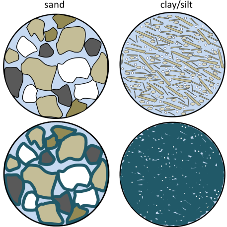
Both sand and clay deposits (and sandstone and mudstone) are quite porous (30% to 50% for sand and 40% to 70% for silt and clay), but while sand can be quite permeable, clay and mudstone are not.
The surface of most silicate mineral grains has a slight negative charge due to imperfections in the mineral structure. Water (H2O) is a polar molecule. This means that while it has no overall electrical charge, one side of the molecule has a slight positive charge (the side with the two hydrogens), compared to a slight negative charge on the other side. Water is strongly attracted to all mineral grains and water within that bound water layer (a few microns around each grain) is not able to move and flow along with the rest of the groundwater. In the lower diagrams shown here, the bound water is represented by dark blue lines around each grain and the water that can move is light blue. In the sand, there is still a lot of water that is able to move through the sediment, but in the clay/silt almost all of the water is held tightly to the grains and this reduces the permeability. [SE]
We have now seen that there is a wide range of porosity in geological materials and an even wider range of permeability. Groundwater exists everywhere there is porosity. However, whether that groundwater is able to flow in significant quantities depends on the permeability. An aquifer is defined as a body of rock or unconsolidated sediment that has sufficient permeability to allow water to flow through it. Unconsolidated materials like gravel, sand, and even silt make relatively good aquifers, as do rocks like sandstone. Other rocks can be good aquifers if they are well fractured. An aquitard is a body that does not allow transmission of a significant amount of water, such as a clay, a till, or a poorly fractured igneous or metamorphic rock. These are relative terms, not absolute, and are usually defined based on someone’s desire to pump groundwater; what is an aquifer to someone who does not need a lot of water, may be an aquitard to someone else who does. An aquifer that is exposed at the ground surface is called an unconfined aquifer. An aquifer where there is a lower permeability material between the aquifer and the ground surface is known as a confined aquifer, and the aquitard separating ground surface and the aquifer is known as the confining layer.
Figure 14.4 shows a cross-section of a series of rocks and unconsolidated materials, some of which might serve as aquifers and others as aquitards or confining layers. The granite is much less permeable than the other materials, and so is an aquitard in this context. The yellow layer is very permeable and would make an ideal aquifer. The overlying grey layer is a confining layer.
The upper buff-coloured layer (K = 10-2 m/s) does not have a confining layer and is an unconfined aquifer. The yellow layer (K = 10-1 m/s) is “confined” by the confining layer (K = 10-4 m/s), and is a confined aquifer. The confined aquifer gets most of its water from the upper part of the hill where it is exposed at the surface, and relatively little by seepage through the fine silt layer.
![Figure 14.4 A cross-section showing materials that might serve as aquifers and confining layers. The relative permeabilities are denoted by hydraulic conductivity (K = m/s). The pink rock is granite; the other layers are various sedimentary layers. [SE]](http://opentextbc.ca/geology/wp-content/uploads/sites/110/2015/08/aquifers-and-confining-layers.png)
Groundwater Flow
If you go out into your garden or into a forest or a park and start digging, you will find that the soil is moist (unless you’re in a desert), but it’s not saturated with water. This means that some of the pore space in the soil is occupied by water, and some of the pore space is occupied by air (unless you’re in a swamp). This is known as the unsaturated zone. If you could dig down far enough, you would get to the point where all of the pore spaces are 100% filled with water (saturated) and the bottom of your hole would fill up with water. The level of water in the hole represents the water table, which is the surface of the saturated zone. In most parts of British Columbia, the water table is several metres below the surface.
Water falling on the ground surface as precipitation (rain, snow, hail, fog, etc.) may flow off a hill slope directly to a stream in the form of runoff, or it may infiltrate the ground, where it is stored in the unsaturated zone. The water in the unsaturated zone may be used by plants (transpiration), evaporate from the soil (evaporation), or continue past the root zone and flow downward to the water table, where it recharges the groundwater.
A cross-section of a typical hillside with an unconfined aquifer is illustrated in Figure 14.5. In areas with topographic relief, the water table generally follows the land surface, but tends to come closer to surface in valleys, and intersects the surface where there are streams or lakes. The water table can be determined from the depth of water in a well that isn’t being pumped, although, as described below, that only applies if the well is within an unconfined aquifer. In this case, most of the hillside forms the recharge area, where water from precipitation flows downward through the unsaturated zone to reach the water table. The area at the stream or lake to which the groundwater is flowing is a discharge area.
What makes water flow from the recharge areas to the discharge areas? Recall that water is flowing in pores where there is friction, which means it takes work to move the water. There is also some friction between water molecules themselves, which is determined by the viscosity. Water has a low viscosity, but friction is still a factor. All flowing fluids are always losing energy to friction with their surroundings. Water will flow from areas with high energy to those with low energy. Recharge areas are at higher elevations, where the water has high gravitational energy. It was energy from the sun that evaporated the water into the atmosphere and lifted it up to the recharge area. The water loses this gravitational energy as it flows from the recharge area to the discharge area.
In Figure 14.5, the water table is sloping; that slope represents the change in gravitational potential energy of the water at the water table. The water table is higher under the recharge area (90 m) and lower at the discharge area (82 m). Imagine how much work it would be to lift water 8 m high in the air. That is the energy that was lost to friction as the groundwater flowed from the top of the hill to the stream.
![Figure 14.5 A depiction of the water table in cross-section, with the saturated zone below and the unsaturated zone above. The water table is denoted with a small upside-down triangle. [SE]](http://opentextbc.ca/geology/wp-content/uploads/sites/110/2015/08/water-table.png)
The situation gets a lot more complicated in the case of confined aquifers, but they are important sources of water so we need to understand how they work. As shown in Figure 14.6, there is always a water table, and that applies even if the geological materials at the surface have very low permeability. Where there is a confined aquifer — meaning one that is separated from the surface by a confining layer — this aquifer will have its own “water table,” which is actually called a potentiometric surface, as it is a measure of the total potential energy of the water. The red dashed line in Figure 14.6 is the potentiometric surface for the confined aquifer, and it describes the total energy that water is under within the confined aquifer. If we drill a well into the unconfined aquifer, the water will rise to the level of the water table (well A in Figure 14.6). But if we drill a well through both the unconfined aquifer and the confining layer and into the confined aquifer, the water will rise above the top of the confined aquifer to the level of its potentiometric surface (well B in Figure 14.6). This is known as an artesian well, because the water rises above the top of the aquifer. In some situations, the potentiometric surface may be above the ground level. The water in a well drilled into the confined aquifer in this situation would rise above ground level, and flow out, if it’s not capped (well C in Figure 14.6). This is known as a flowing artesian well.
![Figure 14.6 A depiction of the water table and the potentiometric surface of a confined aquifer. [SE]](http://opentextbc.ca/geology/wp-content/uploads/sites/110/2015/08/water-table-and-the-potentiometric-surface.png)
In situations where there is an aquitard of limited extent, it is possible for a perched aquifer to exist as shown in Figure 14.7. Although perched aquifers may be good water sources at some times of the year, they tend to be relatively thin and small, and so can easily be depleted with over-pumping.
![Figure 14.7 A perched aquifer above a regular unconfined aquifer. [SE]](http://opentextbc.ca/geology/wp-content/uploads/sites/110/2015/08/perched-aquifer.png)
In 1856, French engineer Henri Darcy carried out some experiments from which he derived a method for estimating the rate of groundwater flow based on the hydraulic gradient and the permeability of an aquifer, expressed using K, the hydraulic conductivity. Darcy’s equation, which has been used widely by hydrogeologists ever since, looks like this:
V = K * i
(where V is the velocity of the groundwater flow, K is the hydraulic conductivity, and i is the hydraulic gradient).
We can apply this equation to the scenario in Figure 14.5. If we assume that the permeability is 0.00001 m/s we get: V = 0.00001 * 0.08 = 0.0000008 m/s. That is equivalent to 0.000048 m/min, 0.0029 m/hour or 0.069 m/day. That means it would take 1,450 days (nearly four years) for water to travel the 100 m from the vicinity of the well to the stream. Groundwater moves slowly, and that is a reasonable amount of time for water to move that distance. In fact it would likely take longer than that, because it doesn’t travel in a straight line.
It’s critical to understand that groundwater does not flow in underground streams, nor does it form underground lakes. With the exception of karst areas, with caves in limestone, groundwater flows very slowly through granular sediments, or through solid rock that has fractures in it. Flow velocities of several centimetres per day are possible in significantly permeable sediments with significant hydraulic gradients. But in many cases, permeabilities are lower than the ones we’ve used as examples here, and in many areas, gradients are much lower. It is not uncommon for groundwater to flow at velocities of a few millimetres to a few centimetres per year.
As already noted, groundwater does not flow in straight lines. It flows from areas of higher hydraulic head to areas of lower hydraulic head, and this means that it can flow “uphill” in many situations. This is illustrated in Figure 14.8. The dashed orange lines are equipotential, meaning lines of equal pressure. The blue lines are the predicted groundwater flow paths. The dashed lines red lines are no-flow boundaries, meaning that water cannot flow across these lines. That’s not because there is something there to stop it, but because there’s no pressure gradient that will cause water to flow in that direction.
Groundwater flows at right angles to the equipotential lines in the same way that water flowing down a slope would flow at right angles to the contour lines. The stream in this scenario is the location with the lowest hydraulic potential, so the groundwater that flows to the lower parts of the aquifer has to flow upward to reach this location. It is forced upward by the pressure differences, for example, the difference between the 112 and 110 equipotential lines.
![Figure 14.8 Predicted equipotential lines (orange) and groundwater flow paths (blue) in an unconfined aquifer. The orange numbers are the elevations of the water table at the locations shown, and therefore they represent the pressure along the equipotential lines. [SE]](http://opentextbc.ca/geology/wp-content/uploads/sites/110/2015/08/unconfined-aquifer.png)
Groundwater that flows through caves, including those in karst areas — where caves have been formed in limestone because of dissolution — behaves differently from groundwater in other situations. Caves above the water table are air-filled conduits, and the water that flows within these conduits is not under pressure; it responds only to gravity. In other words, it flows downhill along the gradient of the cave floor (Figure 14.9). Many limestone caves also extend below the water table and into the saturated zone. Here water behaves in a similar way to any other groundwater, and it flows according to the hydraulic gradient and Darcy’s law.
![Figure 14.9 Groundwater in a limestone karst region. The water in the caves above the water table does not behave like true groundwater because its flow is not controlled by water pressure, only by gravity. The water below the water table does behave like true groundwater. [SE]](http://opentextbc.ca/geology/wp-content/uploads/sites/110/2015/08/limestone-karst-region.png)
Groundwater Extraction
Except in areas where groundwater comes naturally to the surface at a spring (a place where the water table intersects the ground surface), we have to construct wells in order to extract it. If the water table is relatively close to the surface, a well can be dug by hand or with an excavator, but in most cases we need to use a drill to go down deep enough. There are many types of drills that can be used; an example is shown in Figure 14.10. A well has to be drilled at least as deep as the water table, but in fact must go much deeper; first, because the water table may change from season to season and from year to year, and second, because when water is being pumped, the water level will drop, at least temporarily.
![Figure 14.10 A water-well drilling rig in operation in the Cassidy area, near Nanaimo, B.C. In the photo on the right the well is being test-pumped with air pressure. The casing (yellow arrow) is about 40 cm in diameter. [SE]](https://opentextbc.ca/physicalgeologyearle/wp-content/uploads/sites/145/2016/03/well-drilling-2.png)
Where a well is drilled in unconsolidated sediments or relatively weak rock, it has to be lined with casing (steel pipe in most cases) in order to ensure that it doesn’t cave in. A specially designed well screen is installed at the bottom of the casing. The size of the holes in the screen is carefully chosen to make sure that it allows the water to move into the well freely, but prevents aquifer particles from entering the well. A submersible pump is typically used to lift water from within the well up to the where it is needed. The well shown in Figure 14.10 has casing that is about 40 cm in diameter, which might be typical for a municipal water supply well, or a very large well for irrigation. Most domestic wells have 15 cm casing.
Pumping water from the well removes water from inside the well at first. That lowers the water level inside the well. This means that water will flow from the surrounding aquifer (higher groundwater head) toward the pumping well where the groundwater head is now lower. That is how a well gets water from the ground. The water table, or potentiometric surface, will slope in toward the well where the water is being withdrawn. That indicates the energy gradient that is allowing water to flow toward the well. This creates a shape known as a cone of depression surrounding the well, as illustrated in Figure 14.11. If pumping from a well continues for hours to days, the cone of depression may result in a loss of water in nearby wells. As shown in Figure 14.12, pumping of well C has contributed to well B going dry. If pumping continues in well C, it too may go dry.

![Figure 14.12 A similar scenario to that in Figure 14.11, but in this case, wells B and C have been pumped unsustainably for a long time. The cone of depression from well C has reached well B and has contributed to it going dry. [SE]](http://opentextbc.ca/geology/wp-content/uploads/sites/110/2015/08/cone-of-depression.png)
Like other provinces in Canada, British Columbia has a network of observation wells administered by the Ministry of the Environment. These are wells that are installed to measure water levels; they are not pumped. There are 145 active observation wells in B.C. (in 2015), most equipped with automatic recorders that monitor water levels continuously. The main purpose of the observation wells is to monitor water table levels so that we can see if there are long-term natural fluctuations in groundwater quantity, and shorter-term fluctuations related to overuse of the resource. They are also sampled regularly to monitor groundwater chemistry and quality.
An example of an observation well is illustrated in Figure 14.13. This one is situated at Cassidy on Vancouver Island and is used to monitor an unconsolidated aquifer that is widely used by residents with private wells.
![Figure 14.13 B.C. observation well 232 near Cassidy Airport, Vancouver Island. The installation also has a solar panel, which is not visible in this view. [SE]](https://opentextbc.ca/physicalgeologyearle/wp-content/uploads/sites/145/2016/03/obs-well-2.png)
The water-level data from B.C.’s observation wells are available to the public, and an example data set is illustrated in Figure 14.14. The water level in Ministry of Environment observation well 232 (OW-232), situated in Lantzville on Vancouver Island, dropped significantly from 1979 (average depth ~1.5 m), to 2010 (average depth ~5.5 m), but has recovered a little since then.
![Figure 14.14 Water level data for B.C. observation well 232 on Harby Rd., Lantzville, Vancouver Island. From 1979 to 2003, depths were recorded monthly. Automated equipment was installed in 2003, and the depths were recorded hourly since that time. [SE from data at: http://www.env.gov.bc.ca/wsd/data_searches/obswell/map/]](http://opentextbc.ca/geology/wp-content/uploads/sites/110/2015/08/Water-level-data-for-B.C.-observation-well.png)
The short-term variations in the level of well 232 are at a period of one year and are related to annual cycles of recharge and discharge governed by the wet winter climate and drier summers. The data for part of the period are shown in more detail in Figure 14.15. On Vancouver Island, most wells drop to their lowest levels in September or October after the long dry summer period. Levels increase rapidly from October through February as high winter precipitation adds recharge to the aquifer, and water is stored. The water table reaches a peak in March or April. Most wells then drop over the summer as groundwater continues to flow, but no new recharge is added. The water is drained from storage into streams or lakes and eventually into the ocean, and as a result, the water table decreases, reaching its lowest level again in September or October. Similar fluctuations are observed at most observations wells around the province, although the timing is slightly different from region to region.
![Figure 14.15 Water level data for B.C. observation well 232 for the period 1996 to 2000, showing seasonal variations [SE from data at: http://www.env.gov.bc.ca/wsd/data_searches/obswell/map/]](http://opentextbc.ca/geology/wp-content/uploads/sites/110/2015/08/1996-to-2000.png)
The long-term fluctuations in levels in observation wells around the province are also quite variable. Long-term changes in climate can lead to gradual natural changes in water levels. These long-term cycles lasting years or decades are mixed with the effects of well pumping. Some observation wells show consistent decreases in water level that may indicate long-term over-extraction. Many others show generally consistent levels over several decades, and some show increases in water level. One of the important jobs performed by hydrogeologists working for different government ministries is to examine these long-term records of water levels for indications of how sustainable the groundwater use might be.
In 2014, the B.C. government introduced the Water Sustainability Act, which will require licensing groundwater extraction for the first time. This comes into effect in January 2016. The new Act also includes provisions for determining “environmental flow needs” — the amount of water that must be in surface water streams at different times of the year to meet the needs of the ecosystem that depends on the streamflow. For example, many streams in B.C. support populations of salmon that live in the stream for part of their life cycle or return to their home stream for spawning. Groundwater forms a part of the baseflow in a watershed, and is therefore an important part of the environmental flow needs. Careful work is needed in the coming years to ensure that the amount of water licensed to be extracted from surface water and groundwater for human use does not interfere with the amount of water needed for the natural water-dependent ecosystems to function.
The situation in California, where groundwater extraction over large areas is leading to declining water levels, is quite different from that in B.C. According to the state Department of Water Resources, 80% of groundwater wells showed drops in water level of 0 m to 7.5 m between 2011 and 2013, another 6% dropped by 7.5 m to 15 m, and 3% dropped by more than 15 m (Figure 14.16). Over the same time period, only 10% of well levels increased by 0 m to 7.5 m, and 1% increased by more than 7.5 m. The drought that gripped California in 2013 had worsened significantly by 2015, and California farmers — and the people across North America that eat the food they produce — continue to have a prodigious appetite for irrigation water. California, like B.C., is introducing new groundwater regulations to try to control water usage and halt water table declines.
![Figure 14.16 Changes in water levels in wells in California over the period from 2011 to 2013 [SE from State of California Department of Water Resources data]](http://opentextbc.ca/geology/wp-content/uploads/sites/110/2015/08/Changes-in-water-levels.png)
Impermeable Surfaces
Even if groundwater supplies are not being depleted by overuse, or by a changing climate, we are continuing to put stress on aquifers by covering vast areas with impermeable surfaces that don’t allow rain and snowmelt to infiltrate and become groundwater. Instead, water that falls on these surfaces is channelled into drainage systems, then into storm sewers, and then directly into rivers and the ocean. In cities and their suburbs, the biggest culprits are parking lots, roads, and highways. While it would great if we didn’t dedicate such huge areas to cars, that’s not about to change quickly, so we need to think about ways that we can improve surface water infiltration in cities. One way is to use road and parking surfaces that will allow water to seep through, although this is not practical in many cases. Another way is to ensure that runoff from pavement is channelled into existing or constructed wetlands that serve to decontaminate the water, and then allow it to infiltrate into the ground.
Groundwater Quality
As was noted at the very beginning of this chapter, one of the good things about groundwater as a source of water is that it is not as easily contaminated as surface water is. But there are two caveats to that: one is that groundwater can become naturally contaminated because of its very close connection to the materials of its aquifer, and the second is that once contaminated by human activities, groundwater is very difficult to clean up.
Natural Contamination of Groundwater
Groundwater moves slowly through an aquifer, and unlike the surface water of a stream, it has a lot of contact with the surrounding rock or sediment. In most aquifers, the geological materials that make up the aquifer are relatively inert, or are made up of minerals that dissolve very slowly into the groundwater. Over time, however, all groundwater gradually has more and more material dissolved within it as it remains in contact with the aquifer. In some areas, that rock or sediment includes some minerals that could potentially contaminate the water with elements that might make the water less than ideal for human consumption or agricultural use. Examples include copper, arsenic, mercury, fluorine, sodium, and boron. In some cases, contamination may occur because the aquifer material has particularly high levels of the element in question. In other cases, the aquifer material is just normal rock or sediment, but some particular feature of the water or the aquifer allows the contaminant to build up to significant levels.
An example of natural contamination takes place in the bedrock aquifers of the east coast of Vancouver Island and the adjacent Gulf Islands. The aquifer is the Cretaceous (90 Ma to 65 Ma) Nanaimo Group, which is made up of sandstone, mudstone, and conglomerate (Figure 14.17).
The rocks of the Nanaimo Group are not particularly enriched in any trace elements, but the submarine-fan sandstone that makes up much of the group is a lithic wacke, and therefore has relatively high levels of clay (for a sandstone). This clay is good at adsorbing[1] some elements from the water and desorbing others, and in the process, its pH goes up (it becomes alkaline). At high pH levels (some as high as 9 in the Nanaimo Group), the element fluorine that is present naturally in the rock (as it is in almost any rock) has an increased tendency to dissolve in the water. In some areas, groundwater in the Nanaimo Group has fluorine levels that are well above recommended levels for drinking water. The World Health Organization (WHO) maximum acceptable concentration (MAC) for fluorine is 1.5 mg/L (milligrams per litre). Between 5% and 10% of the domestic wells around Nanaimo and adjacent Gabriola Island have more than that, some as much as 10 mg/L. A small amount of fluorine in the human diet is considered important for maintaining dental health, but high levels can lead to malformation and discolouration of teeth, and long-term exposure can lead to other more serious health effects such as skeletal problems.
Nanaimo Group groundwater can also have elevated levels of boron, again related to pH and adsorption from clay minerals. While boron at the levels found there is not toxic to humans, there is enough boron in some wells to be toxic to plants, and the water cannot be used for irrigation.
Rural residents in the densely populated country of Bangladesh (over 1,000 residents/km2, compared with 3.4/km2 in Canada) used to rely mostly on surface supplies for their drinking water, and many of these were subject to bacterial contamination. Infant mortality rates were among the highest in the world and other illnesses such as diarrhea, dysentery, typhoid, cholera, and hepatitis were common. In the 1970s, international agencies, including UNICEF, started a program of drilling wells to access abundant groundwater supplies at depths of 20 m to 100 m. Eventually over 8 million such wells were drilled. Infant mortality and illness rates dropped dramatically, but it was later discovered that the water from a high proportion of these wells has arsenic above safe levels (Figure 14.18).
![Figure 14.18 The distribution of arsenic in groundwater in Bangladesh. The WHO recommended safe level for arsenic is 10 μg/L. All of the green, orange, and red areas on the map exceed that limit. [From: BGS and DPHE. 2001. Arsenic contamination of groundwater in Bangladesh. Kinniburgh, D G and Smedley, P L (Editors). British Geological Survey Technical Report WC/00/19. British Geological Survey: Keyworth. (http://www.bgs.ac.uk/arsenic/bangladesh/) ]](http://opentextbc.ca/geology/wp-content/uploads/sites/110/2015/08/distribution-of-arsenic.png)
[From: BGS and DPHE. 2001. Arsenic contamination of groundwater in Bangladesh. Kinniburgh, D G and Smedley, P L (Editors). British Geological Survey Technical Report WC/00/19. British Geological Survey: Keyworth. (http://www.bgs.ac.uk/arsenic/bangladesh/) ]
Most of the wells in the affected areas are drilled into relatively recent sediments of the vast delta of the Ganges and Brahmaputra Rivers. While these sediments are not particularly enriched in arsenic, they have enough organic matter in them to use up any oxygen present. This leads to water with a naturally low oxidation potential (anoxic conditions); arsenic is highly soluble under these conditions, and so any arsenic present in the sediments easily gets dissolved into the groundwater. Arsenic poisoning leads to headaches, confusion, and diarrhea, and eventually to vomiting, stomach pain, and convulsions. If not treated, the final outcomes are heart disease, stroke, cancer, diabetes, coma, and death. There are ways to treat arsenic-rich groundwater, but it is a challenge in Bangladesh to implement the simple and effective technology that is available.
Anthropogenic Contamination of Groundwater
Groundwater can become contaminated by pollution at the surface (or at depth), and there are many different anthropogenic (human-caused) sources of contamination.
The vulnerability of aquifers to pollution depends on several factors, including the depth to the water table, the permeability of the material between the surface and the aquifer, the permeability of the aquifer, the slope of the surface, and the amount of precipitation. Confined aquifers tend to be much less vulnerable than unconfined ones, and deeper aquifers are less vulnerable than shallow ones. Steeper slopes mean that surface water tends to run off rather than infiltrate (and this can reduce the possibility of contamination). Contamination risk is also less in dry areas than in areas with heavy rainfall.
Studies of groundwater vulnerability have been completed for various regions of British Columbia. A groundwater vulnerability map for southern Vancouver Island is shown in Figure 14.19. The yellow to red areas are considered to have high vulnerability to pollution from surface sources, and most of these are where the aquifers are unconfined in quite permeable unconsolidated sediments of either glacial or fluvial origin, where the water table is relatively shallow and the terrain is relatively flat.
![Figure 14.19 The vulnerability to anthropogenic contamination of aquifers on southern Vancouver Island. Much of the island is not mapped (shown as white) because of a lack of aquifer information in areas without wells. [From: Newton, P. and Gilchrist, A. 2010. Technical summary of intrinsic vulnerability mapping methods of Vancouver Island, Vancouver Island Water Resources Vulnerability Mapping Project, Vancouver Island University, 45pp. Used with permission. https://web.viu.ca/groundwater/PDF/VI_DRASTIC_Summary_Phase2_2010.pdf]](http://opentextbc.ca/geology/wp-content/uploads/sites/110/2015/08/anthropogenic-contamination.png)
The important sources of anthropogenic groundwater contamination include the following:
- Chemicals and animal waste related to agriculture, and chemicals applied to golf courses and domestic gardens
- Landfills
- Industrial operations
- Mines, quarries, and other rock excavations
- Leaking fuel storage tanks (especially those at gas stations)
- Septic systems
- Runoff from roads (e.g., winter salting) or chemical spills of materials being transported
Agriculture
Intensive agricultural operations and golf courses can have a significant impact on the environment, especially where chemicals and other materials are used to enhance growth or control pests. An example of agricultural contamination is in the Abbotsford area of the Fraser Valley, where nitrate levels above the 44 mg/L maximum acceptable level (expressed as nitrate) in the Abbotsford-Sumas aquifer have been observed since the 1950s; however, the problem became much worse as agriculture intensity increased in the 1980s. By 2004, groundwater with nitrate levels in excess of 44 mg/L was reported over an area of about 75 km2 around Abbotsford, and the problem extended across the border into the Sumas area of Washington State.
This region is intensively used for berry crops (especially raspberries and blueberries) and large poultry operations, as well as lesser amounts of grazing and forage crops. Chicken manure is typically stored in fields adjacent to chicken barns, and may release nitrogen to the environment from runoff water, and from releases of ammonia gas. Over decades, both chemical fertilizers and chicken manure and other manures have been applied to the berry crops to provide extra nitrogen to help maximize berry growth. If the fertilizer added is in excess of what the plants need, or is poorly timed compared to when it is needed, then the extra nitrogen may be leached into the groundwater below. Berry crops are irrigated over the summer to help the crops grow. Summer irrigation and winter rainfall may carry excess nitrate from the near surface to the aquifer below.
Since the 1990s, agricultural practices have been tightened up to reduce the rate of groundwater contamination, but it will take decades for nitrate levels to drop in the Abbotsford-Sumas aquifer. Agriculture and Agri-Food Canada and many others are conducting research on better irrigation and nitrate management techniques to reduce the amount of nitrogen that leaches to groundwater.
Landfills
In the past, domestic and commercial refuse was commonly trucked to a “dump” (typically a hole in the ground), and when the hole was filled, it was covered with soil and forgotten. In situations like this, rain and melting snow can easily pass through the soil used to cover the refuse. This water passes into the waste itself, and the resulting landfill leachate that flows from the bottom of the landfill can seriously contaminate the surrounding groundwater and surface water. In the past few decades, regulations around refuse disposal have been significantly strengthened, and important steps have been taken to reduce the amount of landfill waste by diverting recyclable and compostable materials to other locations.
A modern engineered landfill has an impermeable liner (typically heavy plastic, although engineered clay liners or natural clay may be adequate in some cases), a plumbing system for draining leachate (the rainwater that flows through the refuse and becomes contaminated), and a network of monitoring wells both within and around the landfill (Figure 14.20). Once part or all of a landfill site is full, it is sealed over with a plastic cover, and a system is put in place to extract landfill gas (typically a mixture of carbon dioxide and methane). That gas can be sent to a nearby location where it is burned to create heat or used to generate electricity. The leachate must be treated, and that can be done in a normal sewage treatment plant.
![Figure 14.20 A cross-section of a typical modern landfill [SE]](http://opentextbc.ca/geology/wp-content/uploads/sites/110/2015/08/typical-modern-landfill.png)
The monitoring wells are used to assess the level of the water table around the landfill and to collect groundwater samples so that any leakage can be detected. Because some leakage is almost inevitable, the ideal placement for landfills is in areas where the depth to the water table is significant (tens of metres if possible) and where the aquifer material is relatively impermeable. Landfills should also be situated far from streams, lakes, or wetlands so that contamination of aquatic habitats can be avoided.
Today there are hundreds of abandoned dumps scattered across the country; most have been left to contaminate groundwater that we might wish to use sometime in the future. In many cases, it’s unlikely that we’ll be able to do so.
Industrial Operations
Although western Canada doesn’t have the same extent of industrial pollution as other parts of the country, there are still seriously contaminated sites in the west, most with the potential to contaminate groundwater. One example is the lead and zinc smelter at Trail, B.C. The largest in the world, it has been operating for over 100 years and has left a residue of metal contamination around the region (Figure 14.21). In some parts of Trail, the contamination is serious enough that existing soil has been removed from residential properties and replaced with clean soil brought in from elsewhere. This contaminated soil has contributed to contamination of groundwater in the Trail area. Groundwater beneath the actual smelter site is contaminated, and the operator (Teck Resources) is currently working on plans to prevent that water from reaching the nearby Columbia River.
![Figure 14.21 The Trail lead-zinc smelter in 1929 [http://upload.wikimedia.org /wikipedia/commons/2/20 /Trail_Smelter_in_Year_1929.png]](http://opentextbc.ca/geology/wp-content/uploads/sites/110/2015/08/lead-zinc-smelter.png)
[http://upload.wikimedia.org /wikipedia/commons/2/20 /Trail_Smelter_in_Year_1929.png]
Mines, Quarries, and Rock Excavations
Mines and other operations that involve the excavation of large amounts of rock (e.g., highway construction) have the potential to create serious environmental damage. The exposure of rock that has previously not been exposed to air and water can lead to the oxidation of sulphide-bearing minerals, such a pyrite (FeS2), within the rock. The combination of pyrite, water, oxygen, and a special type of bacteria (Acidithiobacillus ferrooxidans) that thrives in acidic conditions leads to the generation of acidity, in some cases to pH less than 2. Water that acidic is hazardous by itself, but the low pH also has the property of increasing the solubility of certain heavy metals. The water that is generated by this process is known as acid rock drainage (ARD). ARD can occur naturally where sulphide-bearing rocks are near the surface. The issue of ARD is a major environmental concern at both operating mines and abandoned mines (see Chapter 20). In streams around the Mt. Washington Mine on Vancouver Island (Figure 14.22), copper levels are high enough to be toxic to fish. Groundwater adjacent to the contaminated streams in the area is very likely contaminated as well.
![Figure 14.22 Acidic runoff at the abandoned Mt. Washington Mine near Courtenay, B.C. [SE]](http://opentextbc.ca/geology/wp-content/uploads/sites/110/2015/08/Acidic-runoff.jpg)
Leaking Fuel Tanks
Underground storage tanks (USTs) are used to store fuel at gas stations, industrial sites, airports, and anywhere that large volumes of fuel are used. They do not last forever, and eventually they start to leak their contents into the ground. This is a particular problem at older gas stations — although it may also become a future problem at newer gas stations. You may have noticed gas stations that have been closed and then surrounded by chain-link fence (Figure 14.23). In virtually all such cases the closure has been triggered by the discovery of leaking USTs and the requirement to cease operations and remediate the site.
![Figure 14.23 A closed and fenced gas station site in Nanaimo, B.C. The white pipes in the background are wells for monitoring groundwater contamination on the site. [SE]](http://opentextbc.ca/geology/wp-content/uploads/sites/110/2015/08/fenced-gas-station-site.jpg)
Petroleum fuels are complex mixtures of hydrocarbon compounds and the properties of their components — such as density, viscosity, solubility in water, and volatility — tend to vary widely. As a result, a petroleum spill is like several spills for the price of one. The petroleum liquid slowly settles through the unsaturated zone and then tends to float on the surface of the groundwater (Figure 14.24). The more readily soluble components of the spill dissolve in the groundwater and are dispersed along with the normal groundwater flow, and the more volatile components of the spill rise toward the surface, potentially contaminating buildings.
![Figure 14.24 A depiction of the fate of different components of a petroleum spill from an underground storage tank. [SE]](http://opentextbc.ca/geology/wp-content/uploads/sites/110/2015/08/petroleum-spill.png)
Septic Systems
In areas that are not served by sewage networks leading to a central sewage treatment plant, most homeowners rely on septic systems for disposal of sewage. There are two primary components to a simple septic system, the septic tank and the drainage field (Figure 14.25). A typical septic tank is constructed of either concrete or plastic and has a volume of 5,000 L to 10,000 L (5 m3 to 10 m3). This forms the first treatment and is designed to be anaerobic (without oxygen). That promotes the activity of certain bacteria that help break down the waste. As the waste is degraded, some portions tend to sink to form sludge at the base of the tank, and others float to the surface, forming a scum layer. A septic tank may be divided into two parts to keep the sludge at the bottom and the scum on the top from draining out. The water then moves to the drainage field, which provides the right conditions for a different set of bacteria that operate in aerobic conditions. The drainage field includes an array of plastic pipes that are perforated to allow the effluent to drain out over a large area and seep slowly into the ground. In order to install a drainage field, it is first necessary to test the soil below, as it must be sufficiently permeable to allow the effluent to percolate away, but not so permeable that it flows too quickly and the soil is not able to filter out the pathogenic bacteria.
If they are properly installed and used, and if the sludge is periodically removed from the tank, a septic system should be effective in treating the sewage for decades. The anaerobic and aerobic bacteria should be able to break down the incoming waste and there should be little risk to the surface environment or groundwater. But many things can go wrong with a septic system, including the following:
- If inappropriate chemicals are added to the waste stream, they may interfere with the natural breakdown of the sewage.
- If the tank is not periodically pumped out, solids can get into the drainage field and compromise the drainage, resulting in the flow of effluent toward the surface.
- If the soil is either not sufficiently permeable or too permeable, the effluent will not drain away (and will start to pool at the surface) or it will drain too quickly.
- If the drainage field is constructed in an area where the water table is close to surface, some of the effluent is likely to flow into the groundwater without being treated.
![Figure 14.25 A typical septic system. [SE]](http://opentextbc.ca/geology/wp-content/uploads/sites/110/2015/08/septic-system.png)
Prevention and Mitigation of Groundwater Contamination
As illustrated in the landfill example above, there are two fairly simple ways to significantly reduce the chance and degree of groundwater contamination from surface sources. One is to prevent rainwater from infiltrating down to the water table and picking up contaminants; this can be achieved by simply capping or roofing over the landfill, mine tailings, or spill site. The second is to provide an impermeable barrier beneath the contaminant. Modern landfills and mine tailings impoundments are all built using some combination of clay and engineered plastic barriers. Both of these solutions — caps and liners — are subject to failure due to leaks.
Once contaminants are in the groundwater, the main form of remediation is to pump out the contaminated water and treat it at the surface. This can be a slow process, and preventing the contaminant from travelling significantly during this process can be accomplished by manipulating local groundwater flow through the extraction or injection of water at certain locations. Consider this in the exercise below.
Summary
The topics covered in this chapter can be summarized as follows:
| 14.1 | Groundwater and Aquifers | Porosity is the percentage of open space within a rock or unconsolidated sedimentary deposit, while permeability is the facility with which water can be transmitted through that material. An aquifer is a body of rock or sediment that has sufficient permeability for water to be extracted, while an aquitard is an impermeable body. An aquifer is described as confined if it is overlain by an impermeable layer (confining layer), or unconfined if it has no such confining layer. |
|---|---|---|
| 14.2 | Groundwater Flow | The water table is the upper surface of the saturated zone in an unconfined aquifer. A confined aquifer has a potentiometric surface (instead of a water table), which is defined as the level to which water would rise if a well were drilled into the confined aquifer. Change in groundwater head over distance is the hydraulic gradient. The theoretical velocity of flow in an aquifer is defined by Darcy’s law as the hydraulic conductivity (a measure of permeability) times the hydraulic gradient (V = K * i). It is possible to predict groundwater flow paths if we can draw equipotential lines within an aquifer. In areas where limestone has solutional openings (e.g., caves), water flow is determined by gravity above the water table and by the hydraulic gradient below the water table. |
| 14.3 | Groundwater Extraction | Groundwater can be extracted at springs, but in most cases, wells are needed to ensure a steady supply. Pumping groundwater from a well lowers groundwater head near the well, creating flow toward the well. This creates a cone of depression around the well. Excessive pumping can lead to a well running dry or to a lack of water in nearby wells. During extended periods of dry weather, or if consistent over-pumping occurs, aquifers may be depleted. Observation wells are used to monitor short-term and long-term changes in water levels that can indicate changes in aquifer health. |
| 14.4 | Groundwater Quality | The quality of groundwater can be compromised by both natural and anthropogenic contamination. Natural contamination can be caused by particularly high levels of contaminants within the aquifer itself, but is more commonly a result of enhanced solubility of contaminants due to the aquifer chemistry. Some common sources of anthropogenic contamination include agriculture, industry, mining, landfills, and leaking underground storage tanks. We can assess the vulnerability of aquifers to contamination by mapping regional variations in parameters such as depth to the water table, permeability, slope, and precipitation. |
- “Adsorb” (with a “d”) is not the same as “absorb” (with a “b”). Water can be absorbed by a sponge. Ions dissolved in water can be adsorbed onto — or desorbed from — the surfaces of clay minerals. ↵

Feedback/Errata