Thermodynamics of the Solvation of Salts

Yu Kay Law

10 Thermodynamics of the Solvation of Salts

Yu Kay Law

Purpose

To determine $\Delta H^\circ$ , and $\Delta S^\circ$ for the solvation of different salts.

Expected Learning Outcomes

Define and measure the solubility product constant for a salt at different temperatures.
Determine thermodynamic parameters associated with chemical equilibria.

Textbook Reference

Tro, Chemistry – Structures and Properties, 2nd Ed, Ch. 17.5 (K_sp) and 18.9 (Gibbs energy and chemical equilibria).

Introduction

Describing Solubility Using the Language of Chemical Equilibria

In the chapter on solubility, we described the solubility in terms of the mass of solute dissolved per 100 g of solvent. Fairly straightforwardly, we can also quantify the solubility by the molarity of a saturated solution: the molar solubility.

The diagram shows eight purple spheres labeled K superscript plus and eight green spheres labeled C l superscript minus mixed and touching near the center of the diagram. Outside of this cluster of spheres are seventeen clusters of three spheres, which include one red and two white spheres. A red sphere in one of these clusters is labeled O. A white sphere is labeled H. Two of the green C l superscript minus spheres are surrounded by three of the red and white clusters, with the red spheres closer to the green spheres than the white spheres. One of the K superscript plus purple spheres is surrounded by four of the red and white clusters. The white spheres of these clusters are closest to the purple spheres. — Dissociation of sodium chloride in aqueous solution.

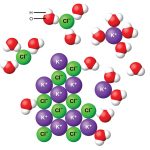
For an ionic compound, when it dissolves it would dissociate into its constituent ions. For a slightly soluble compound such as potassium dichromate (K₂Cr₂O₇), for example,

(1) $\begin{equation*} \ce{K2Cr2O7}(s) \rightleftharpoons 2\ce{K+}(aq) + \ce{Cr2O}_7^{2-}(aq) \end{equation*}$

where we treat the process as an equilibrium process. With the solvation process being treated as an equilibrium, we can write its equilibrium constant as

(2) $\begin{equation*} K_{\textrm{sp}} = [\ce{K+}]^2 [\ce{Cr2O}_7^{2-}] \end{equation*}$

where we call the equilibrium constant for the dissociation of an ionic compound in solution the solubility-product constant K_sp. Given the molar solubility, we can find the K_sp value using an ICE table as we did in Ch. 15. This is further explained in the following video:

https://iu.mediaspace.kaltura.com/id/1_31k4k1ff?width=400&height=285&playerId=26683571

Gibbs Free Energy and the Equilibrium Constant

The Gibbs Free Energy

We know that, for a spontaneous process under constant pressure and temperature, the Gibbs energy of a process, defined as

(3) $\begin{equation*} \Delta G = \Delta H - T \Delta S \end{equation*}$

would decrease. Furthermore, at equilibrium, it can be shown that $\Delta G = 0$ . Furthermore, it can be shown that the standard Gibbs free energy is related to the equilibrium constant by

(4) $\begin{equation*} \Delta G^\circ = -RT \ln K \end{equation*}$

Here, the degree sign in $\Delta G^\circ$ denotes that this is the standard Gibbs free energy change, where standard refers to standard conditions: solutes have a molarity of 1 M and gases have a partial pressure of 1 atm.

Assuming that $\Delta H^\circ$ and $\Delta S^\circ$ are temperature-independent, we can relate the equations above to yield the equation

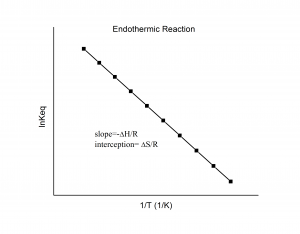
(5) $\begin{equation*} \ln K = - \frac{\Delta H^\circ}{R} \times \frac{1}{T} + \frac{\Delta S^\circ}{R} \end{equation*}$

Van't Hoff plot for an endothermic reaction. — van’t Hoff plot for an endothermic reaction

where $R = 8.314\textrm{ J}/\textrm{mol}\cdot \textrm{K}$ is the ideal gas constant. From this equation, you can show that if you plot ln K (along the y-axis) against 1/T (along the x-axis, with temperature in Kelvins) you should yield a straight line with the slope being $\Delta H/R$ and the y-intercept being $\Delta S/R$ .

In this experiment, you will measure the $K_{\textrm{sp}}$ for two different salts at different temperatures. You will then find $\Delta H^\circ$ and $\Delta S^\circ$ of the solvation process.

Procedure

You will perform this experiment using the ChemCollective Temperature and the Solubility of Salts virtual lab – it’s unrealistic but it would illustrate the chemical concepts.

Each student will study the solubility of three solids: cerium sulfate (Ce₂(SO₄)₃; there is a typo in the name on the Virtual Lab) and two others to be assigned by your instructor. For each solute, you will determine the molarity of each ion of a saturated solution at a number of different temperatures (at least five per solute) as follows:

Obtain distilled water and measure out 20 mL into a 250 mL beaker.
Get a foam cup (from Glassware > Other) ready.
Heat the water to the desired temperature in the beaker, and then pour the water quickly into the foam cup.
Add the desired solid into the cup until there is solid (as shown in the information tab on the left).
“Filter” the solution by right clicking on the foam cup and selecting “remove solid”.
Record the molarities of the cation and anion, along with the temperature of the contents of the foam cup (which will not be the same as the temperature of the water you had).

Even for room temperature, it is important that you dissolve the solid in the foam cup or it takes a while for the concentration to equilibrate due to the change in temperature.

You can then use this information to create a van’t Hoff plot as described above, and then obtain $\Delta H^\circ$ and $\Delta S^\circ$ for this process.