Beer’s Law Virtual Lab

Yu Kay Law

14 Beer’s Law Virtual Lab

Expected Learning Outcomes

After completing this experiment, students are expected to be able to

Relate the color of a solution to its absorption spectrum. (LO 5)
Measure the absorption spectrum of a substance. (LO 3)
Make Beer’s Law plots and use the plot to find the concentration of a sample. (LO 3, 4, 6)

Textbook Reference

Tro, Chemistry: Structures and Properties, 2nd Ed, Ch. 8.2.

Introduction

Absorption of Light

As we saw in our discussion of spectroscopy related to our research project a few weeks ago, when light passes through a sample, some proportion of the light will be absorbed, depending on the electronic structure of the molecule^[1] and the wavelength of the incoming light, while the rest of the light is transmitted. In the figure below, the incident (incoming) light intensity is $I_0$ and the transmitted light intensity (the light that is able to make it through the sample and out the other side) is $I_t$ .

To quantify this, we note that – at a particular wavelength – given that the intensity of incident light is $I_0$ , the intensity of light that goes through the sample is $I_1$ ; the rest of this light is absorbed by the sample:

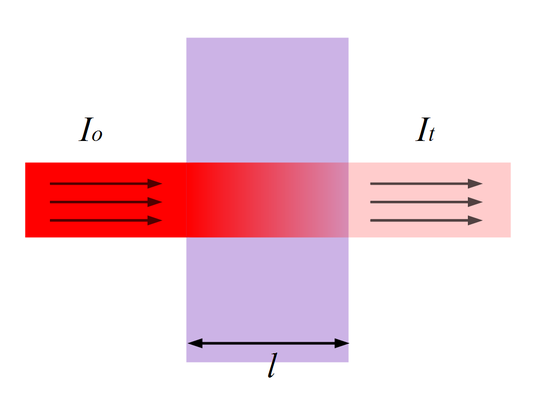
light with intensity I0 enters cuvette; less light I1 exits cuvette after path length of l — Transmission of light through.a cuvette. Credit: Heesung Shim/Libretexts.

To quantify the amount of light that is absorbed, we define the absorbance ( $A$ ) as

(1) $\begin{equation*} \frac{I_1}{I_0} = 10^{-A} \to A = -\log_{10}\left(\frac{I_1}{I_0}\right) \end{equation*}$

Note that the absorbance is unitless.

In this case, we can plot an absorption spectrum – a graph of the absorbance ( $A$ ) as a function of the wavelength of a sample:

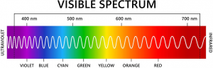
Note that the absorbance varies with both concentration and wavelength for a given substance.

plot of molar extinction coefficient vs wavelength. Peak is around 620 nm — Absorption spectrum of methylene blue. Credit: Scott Prahl.

The color of the solution will be the complementary color of the color of light being absorbed – which is the color opposite the wavelength of light in the color wheel:

Colors arranged in a circle - the color wheel. — Color wheel. Credit: Marian Sigler/Wikimedia.

Examples

Methylene blue absorbs primarily at around 620 nm, which corresponds to orange on the visible spectrum. This is opposite to blue on the color wheel, and aligns with the solution.

The visible spectrum is as follows:

The visible spectrum with colors and wavelengths. — The visible part of the electromagnetic spectrum. Credit: Elena Pimukova.

The absorbance of a solution can be measured using a spectrophotometer; details on how to use this is explained in Using Laboratory Equipment.

Beer-Lambert Law

It can be shown that for a solution with a concentration (molarity) of $c$ ,^[2] the absorbance is related to this by

$A = \varepsilon cl$

where $l$ is the path length (the thickness of the solution through which the light travels; this is typically reported in centimeters) and $\varepsilon$ is the molar absorptivity (with units of $\mbox{M}^{-1}\mbox{cm}^{-1}$ ). The molar absorptivity varies with wavelength, and is a property of a particular substance at a given wavelength.

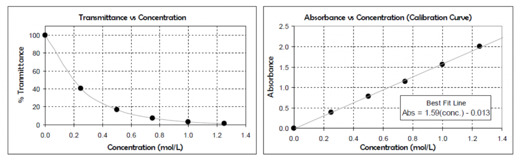
A plot of transmittance vs concentration (exponential decay) and absorbance vs concentration (straight line upwards. — The transmittance and the absorbance of a solution as a function of concentration. Credit: Stephen Donnelly, Fort Hays State University.

The molar absorptivity at a given wavelength can be found by producing a Beer’s Law plot (like on the right hand side of the figure above). To do this, solutions of different concentrations of the compound being studied are prepared and their absorbances at the chosen wavelength are plotted (along the y-axis) against the concentrations of these solutions (along the x-axis).

Based on this, the molar absorptivity ε can be found from the slope of the Beer’s Law plot. The slope of the Beer’s Law plot is equal to $\varepsilon l$ . Most cuvettes used in the laboratory have a 1 cm pathlength, and therefore in your experiment you can use this to find the molar absorptivity. Remember that typically Beer’s Law is set up with units such that the path length is in cm.

Using the molar absorptivity, we can determine the concentration of an unknown solution of the same compound^[3] by measuring the absorbance of the sample at the same wavelength as was done for the standard solutions. Given the molar absorptivity found from the Beer’s Law plot, one can solve Beer’s Law to find the absorbance.^[4]

This technique is very widely used in modern analytical chemistry and is one of the primary ways, for example, by which proteins and nucleic acids are quantified in the biochemical laboratory.

Dilution Calculations

Often, in chemistry, we start with more concentrated stock solutions and dilute these to get the concentration we want. This is a key skill that you should acquire. We do this quite often with concentrated drinks as well.

When we dilute a stock solution with a volume $V_1$ by a molarity $M_1$ with the solvent such that the final volume of the solution is $V_2$ , the molarity of the diluted solution can be related to the other quantities by

(2) $\begin{equation*} M_1 V_1 = M_2 V_2 \end{equation*}$

In this equation $V_2$ is the total volume of the final solution, not the volume of the solvent added!

This equation could also be used to back-solve the concentration of a stock solution from that of a diluted solution. Be aware that this equation can only be used when you are diluting something (i.e. when you add water to a SOLUTION to decrease that solutions concentration). It cannot be used to calculate the concentration when you dissolve a SOLID (or a pure liquid instead of a solution) in water.

Example: if you take 32.6 mL of a 0.53 M NaCl solution and dilute it to 99.3 mL with distilled water (i.e. the total volume of NaCl solution + distilled water = 99.3 mL), we can calculate the molar concentration of the diluted solution using M₁V₂=M₂V₂. M₁ = the molar concentration of the stock solution (0.53 M NaCl in this example). V₁ = the volume of the stock solution that was used to make the diluted solution (32.6 mL in this example). M₂ = the molar concentration of the diluted solution (what we’re trying to find in this example). V₂ = the total volume of the diluted solution (99.3 mL in this example). When we plug these numbers in, we get 0.53 M NaCl * 32.6 mL = X M NaCl * 99.3 mL. This can then be rearranged to isolate M₂: X M NaCl = (0.53 M NaCl * 32.6 mL)/99.3 mL = 0.17 M NaCl.

Procedures

Keep the results of this experiment in your laboratory notebook as you will need this information in CHEM-C 126.

Obtaining the Absorption Spectrum for a Drink Mix (Allura Red)

In this part of the experiment, you will collect the absorption spectrum of Allura Red using this PhET simulation.

Go to the PhET simulation above and select “Beer’s Law”.
Change from “Transmittance” to “Absorbance” and from “Preset” to “Variable”, then adjust the wavelength all the way to the left (380 nm). (Make sure the “Solution” is still on the default of “Drink mix”.)
Turn on the laser on the left of the screen by pressing the red button.
Measure the absorbance from 380 nm to 780 nm every 20 nm (i.e., 380, 400, 420, 440, etc.).
Wherever the absorbance is highest, measure the absorbance 10 nm above and below that wavelength every 2 nm.
- For example, if you find that the highest absorbance is at 620 nm, then measure the absorbance at 610, 612, 614, 616, 618, 622, 624, 626, 628 and 630 nm.
Plot the absorbance vs wavelength on Excel.
1. Put the wavelength in column 1 (in order of smallest to highest wavelength)
2. Put the absorbance of the corresponding wavelengths in column 2
3. Select the data in both columns by clicking and dragging over both columns
4. Go to Insert, Chart, Scatterplot with smooth lines. This should create a scatterplot with wavelength on the x-axis and absorbance on the y-axis.
5. Add an appropriate chart title and axis title for both the x- and y-axes (including the units used) by going to the “Chart Design” tab at the top and clicking on “Add Chart Element”, “Axis Titles” and selecting “Primary Horizontal” and “Primary Vertical”.
Determine the best wavelength (i.e. the wavelength that gives the highest absorbance) at which you should measure the absorption values for the Beer’s Law plot.

Creating the Beer’s Law Plot

In this part of the experiment, you will create a Beer’s Law plot by determining the concentration of drink mix needed to give specific absorbances and then plot your results in Excel.

Change the wavelength of the laser to the wavelength determined in step 7 of the previous part of the experiment, then adjust the concentration of the drink mix so that the absorbance is 0.00.
Record the millimolar (mM) concentration of the drink mix at this absorbance.
Repeat steps 1 and 2 for an absorbance of 0.25, 0.50, 0.75, and 1.00
Plot the absorbance vs concentration in Excel.
1. Put the molarity of each solution in column 1
2. Put the absorbance for the corresponding solutions in column 2
3. Select the data in both columns by clicking and dragging over both columns
4. Go to Insert, Chart, Scatterplot. This should create a scatterplot with concentration on the x-axis and absorbance on the y-axis.
5. Right click on one of the data points and select “trendline”. This should add a best-fit-line to your plot.
6. Right click on the line and select “Format Trendline”,
7. Check the “Display Equation on chart” and “Display R-squared value on chart” boxes. The slope of the best-fit-line is the molar absorptivity of Allura red.
8. Add an appropriate chart title and axis title for both the x- and y-axes (including the units used) by going to the “Chart Design” tab at the top and clicking on “Add Chart Element”, “Axis Titles” and selecting “Primary Horizontal” and “Primary Vertical”.

Preparation and Absorbance of Dilute Solutions

In this part of the lab, you will need to use the best-fit-line equation of your Beer’s Law plot to figure out what concentration of Allura red is needed to give an absorbance of 0.93 and then attempt to make that solution by diluting a stock solution 5 times.

Take the best-fit-line of your Beer’s Law plot from the previous part of this lab and calculate what concentration of Allura red is needed to give an absorbance of 0.93 (remember that y for our plot is absorbance and x is mM).
Go to the “Concentration” portion of the PhET simulation (found at the bottom of the screen).
Change the “Solute” in the top right from “Solid” to “Solution” (make sure it is still on the default “Drink mix”).
Empty all the water in the beaker by pulling on the valve of the drain at the bottom right of the beaker.
Add ~0.1 L of drink mix solution to the beaker by pressing the red button at the top of the dropper.
Record the appearance of the stock solution.
Move the probe (circle with crosshairs) on the “Concentration” meter so that the center of the probe is over the stock solution, then read the concentration off the meter (M1).
Use M₁V₁=M₂V₂ to calculate the volume of the stock solution (V1) needed to give the concentration of Allura red (M2) needed to give an absorbance of 0.93 as calculated in step 1 above if you dilute to 1 L (V2).
Drain all of the solution from the beaker.
Add the amount of stock solution you calculated in step 8 above to the beaker to the best of your ability given the precision of the beaker.
Dilute the stock solution to 1.000 L by opening the valve on the faucet at the top right until the beaker is completely full.
Measure the concentration of this dilute solution.
Move back to the Beer’s Law portion of the simulation and change the concentration of Allura red in the cuvette to the concentration you measured in step 12 (make sure the wavelength is still at the peak absorbance you measured in part 1 above and the “Solution” is still set to “Drink mix”).
Record the absorbance of the solution at this concentration
Repeat steps 9-14 four more times so that you have 5 concentration and absorbance measurements.

The discussion on this is rather complex and is well beyond the scope of this course, but it is related to 2 topics taught in CHEM-C 105: atomic absorption spectroscopy and resonance and some discussion of how this impacts what wavelengths a molecule absorbs is had in the CHEM-C 344 organic chemistry laboratory course. ↵
While we will use molarity for this purpose in this class, in principle you can use any concentration unit. It will just alter the units/numerical value of ε. ↵
In the same solvent, in principle, though the absorption spectrum doesn't vary too much as a function of solvent in many cases. ↵
You should, however, be aware that Beer's Law only works for relatively low concentrations. Beyond an absorbance of about $A = 1.5$ , Beer's Law breaks down. ↵