Purpose

Determine the heat of fusion of ice and the heat of reaction for a chemical reaction.

Expected Learning Outcomes

After completing this experiment, students should be able to measure the enthalpy change associated with physical and chemical changes.

Textbook Reference

Tro, Chemistry: Structures and Properties, 2nd Ed, Ch. 9.4, 9.7 (calorimetry and thermal energy transfer) and 11.6-7 (enthalpy changes of phase changes)

Introduction

Enthalpy Changes Associated with Physical and Chemical Changes

In chemistry, all processes are associated with the transfer of energy between the system and the surroundings. Under constant pressure conditions, we typically experience this through the transfer of heat – which is associated with changes in temperature. The heat ([latex]q[/latex]) associated with a process is related to temperature change by^[1]

[latex]q = m C_S \Delta T[/latex]

where [latex]C_S[/latex] is the specific heat capacity of a substance.  Under constant pressure conditions (most of the time), the heat associated with a process is equal to its enthalpy change.  Therefore, by determining the heat associated with a process, we can find the enthalpy change.

Important types of enthalpy changes include:

• The heat of reaction [latex]\Delta H_{\mbox{rxn}}[/latex] is the enthalpy change associated with a particular reaction following its thermochemical equation.

• The heat of fusion, [latex]\Delta H_{\textrm{fus}}[/latex] is the enthalpy change associated with melting a particular substance from solid to liquid. This is typically reported in units of kJ/mol – i.e. the heat (in kilojoules) required to melt one mole of the substance.  At this level, we will assume this occurs at the freezing point.
• Similarly, the heat of vaporization [latex]\Delta H_{\mbox{vap}}[/latex] is the enthalpy change associated with vaporizing a liquid. Again, this is typically reported in kJ/mol – the amount to vaporize one mole of a liquid.

Sign Conventions for Enthalpy Changes

Reactions can either require heat input for the process to occur (it takes in heat, such as for a cold pack) or transmit heat to the surroundings (such as when dynamite explodes). We can therefore classify processes as exothermic or endothermic.^[2]  Furthermore, chemists are interested in the energy change of the system, and therefore we define our signs in terms of changes experienced by the system (as we will do throughout our study of thermodynamics).

• Endothermic processes take in heat – it requires heat to be transferred from the surroundings into the system (mixture of reactants and products).  In this case, the system gains energy through heat and the sign of [latex]\Delta H[/latex] is positive.

• Exothermic processes give off heat – it evolves heat.  In this case, the system loses energy through heat and therefore the sign of [latex]\Delta H[/latex] is negative.

Calorimetry

Calorimetry is the art of measuring the enthalpy change when a physical or chemical change occurs. In this course, you will use a coffee-cup calorimeter to measure the following enthalpy changes:

• The heat of fusion [latex]\Delta H_{\mbox{fus}}[/latex] of ice.
• The heat of reaction [latex]\Delta H_{\textrm{rxn}}^\circ[/latex] for the single displacement reaction of hydrochloric acid with magnesium metal

[latex]\ce{Mg}(s) + 2\ce{HCl}(aq) \to \ce{MgCl2}(aq) + \ce{H2}(g)[/latex]

In both cases, you will measure the temperature change associated with the process, from which the heat of fusion or heat of reaction will be determined using the equation

[latex]q = m C_S \Delta T[/latex]

as well as your knowledge of the masses of solutions present. You can then compare these results with those derived from heats of formation or other reference values reported in reference works such as the CRC Handbook of Chemistry and Biology or the NIST Chemistry WebBook.

For this experiment, we will be assuming that the heat capacity of the calorimeter is zero. In reality, the coffee-cup calorimeter will absorb heat and this will be a source of error in our calculations in this experiment.^[3]

Procedures

Special Equipment Needed

• Four 250 mL coffee cups with two lids.
• Vernier Temperature probe.  You will need a device (cellphone/tablet/etc) equipped with Vernier Graphical Analysis.
• Sandpaper
• Stir bar

Part A: Heat of Fusion of Ice

In this part, you will attempt to use hot water to melt a sample of ice. The goal is to find the mass of ice required to cool the hot water from about 60°C to about 4″C. From this, and applying the Law of Conservation of Energy as well as the accepted value for the specific heat capacity of liquid water ([latex]C_S=4.184 \text{ J}/\text{g}\cdot\text{K}[/latex]) and for ice ([latex]C_S = 2.10 \text{ J}/\text{g}\cdot\text{K}[/latex]), we can determine the heat of fusion of water.

Procedures

1. Turn on the Vernier Graphical Analysis app on your device and connect the provided temperature probe to the app.
2. Make two calorimeters. Each calorimeter is produced by stacking two coffee cups together.
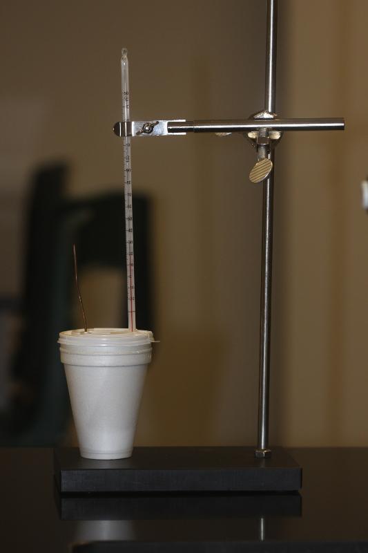
3. Measure in a graduated cylinder approximately 50 mL of deionized water. Pour the deionized water into a 250 mL beaker and heat this water to approximately 60°C. Use the thermometer to check the temperature from time to time.
4. Fill one of the two calorimeters with ice cubes, and measure the initial temperature of the ice cubes ([latex]T_C[/latex]) using the temperature probe. To do this:
   1. Place the probe into the calorimeter. At the bottom right hand corner of the interface the temperature will be displayed (in a small box).
   2. Once the value has mostly stabilized, click on “collect” to collect the data. After you’ve allowed the data to stabilize, click on “keep”.
5. To find the average value, click on the Graph Tools icon near the bottom left corner. Click on the statistics option, which will display various statistics for the temperature values. Record the average value.  After this is done, you may reset the experiment.
6. Measure the mass of the calorimeter containing ice cubes.
7. When the hot water is ready, transfer the hot water from the beaker into the second (empty except for a stir bar) calorimeter. Record the temperature of this water as described in Step 4 above.

8. Open the lid of the calorimeter containing hot water and place one or two ice chips into the hot water. Collect the temperature values.
9. Stir the water and allow the ice chips to melt.
10. As the ice chips melt, add more ice chips to ensure that there is always some solid ice chips remaining in the water.

11. As the temperature approaches 6°C, stop adding ice chips and close the lid. Allow the temperature to stabilize and measure the final, equilibrated temperature of the calorimeter ([latex]T_f[/latex]) following the directions in step 4.
12. Determine the mass of the calorimeter containing the ice chips. By subtracting this from the initial mass of the calorimeter full of ice chips, you can determine the mass of ice added to the other calorimeter.

Data Analysis

The goal of this part of the experiment is to find the heat of fusion of water, [latex]\Delta H_{\mbox{fus}}^\circ[/latex]. To analyze this situation, we need to consider the heating curve for the ice.

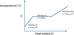
The figure above shows that the ice can potentially undergo up to three distinct processes:

• The ice was heated to the freezing point of water (0°C). The heat required is \begin{equation}q_1 = m_{\mbox{ice}}\times C_{S,\mbox{solid}} \times \Delta T_1\end{equation} where the specific heat capacity of ice, [latex]C_{S,\mbox{solid}} = 2.10 \text{ J}/\text{g}\cdot \text{K}[/latex], [latex]\Delta T_1[/latex] is the change in temperature from the initial temperature [latex]T_C[/latex] to 0°C (i.e. [latex]\Delta T_1 = 0^\circ\textrm{C} - T_C[/latex]). If the ice was already at (or above^[4]) the freezing point then this process would not occur, and should be neglected.
• The ice was melted at the freezing point. This is related to the heat of fusion by \begin{equation}q_2 = n\Delta H_{\mbox{fus}}^\circ\end{equation} where n is the number of moles of ice that was molten. Since the goal is to determine [latex]\Delta H_{\mbox{fus}}^\circ[/latex], we will leave this term alone for now.
• The ice was heated to the freezing point of water (0°C). The heat that is transferred into the (former) ice is
  \begin{equation}
  q_3 = m_{\mbox{ice}}\times C_{S,\mbox{water}} \times \Delta T_3
  \end{equation}
  where the specific heat capacity of water is [latex]C_{S,\mbox{water}} = 4.184 \text{ J}/\text{mol}\cdot \text{K}[/latex] and [latex]\Delta T_3[/latex] is the temperature change of the original ice from the freezing point of water (0°C) to the final temperature [latex]T_f[/latex] (i.e. [latex]\Delta T_3 = T_f - 0^\circ\textrm{C}[/latex]).

Therefore, the heat gained by the ice is the sum of the three terms above
\begin{equation}
q_{\mbox{ice}} = q_1 + q_2 + q_3
\end{equation}

Assuming a perfect calorimeter (i.e. there is no transfer of heat out of the coffee cup calorimeter), the heat gained by the ice must come from the water.
\begin{equation}
q_{\mbox{ice}} = -q_{\mbox{water}} \label{360:qcons}
\end{equation}
where the negative sign indicates that the heat is transferred \emph{away} from the water. $q_{\mbox{water}}$ can be determined using the expression
\begin{equation}
q_{\mbox{water}} = m_{\mbox{water}} \times C_{S,\mbox{water}} \times \Delta T_{\mbox{water}}
\end{equation}
where [latex]m_{\mbox{water}}[/latex] is the mass (in g) of the hot water and [latex]\Delta T_{\mbox{water}}[/latex] is the change in temperature of the hot water from the initial (maximum) temperature [latex]T_H[/latex] to the final, equilibrated temperature [latex]T_f[/latex], such that [latex]\Delta T_{\mbox{water}} = T_f - T_H[/latex]. The mass of water can be found based on the volume of water recorded and the density of water (1.00 g/mL).^[5]

As the final temperature is lower than the initial temperature, [latex]\Delta T_{\mbox{water}}[/latex] is negative, and hence [latex]q_{\mbox{water}}[/latex] would be negative as well.

Based on the above, we can show that

\begin{equation}-q_{\mbox{water}} = q_1 + q_2 + q_3\end{equation}

\begin{equation}q_2 = -q_{\mbox{water}} – q_1 – q_3\end{equation}

where the values of [latex]q_{\mbox{water}}[/latex], [latex]q_1[/latex] and [latex]q_3[/latex] can be found as described above. The value of [latex]q_2[/latex] can then be used to find the heat of fusion of water [latex]\Delta H_{\textrm{fus}}^\circ[/latex].

Part B: Enthalpy Change in a Single Displacement Reaction

In this part of the experiment, you will react a strip of magnesium ribbon with hydrochloric acid

[latex]\ce{Mg}(s) + 2\ce{HCl}(aq) \to \ce{MgCl2}(aq) + \ce{H2}(g)[/latex]

Procedure

13. Rinse, clean and dry the calorimeters and thermometers you have used so far.
14. Take a strip of magnesium metal and sand it down if there any of it appears to be oxidized until all of the tarnish has come off.
15. Determine the mass of the strip of magnesium metal. It should be approximately 0.12 g; if it is less than 0.10 g then you will need some more.
16. Measure and add about 60.0 mL of 2.0 M hydrochloric acid using a graduated cylinder to the calorimeter. Place a clean, dry stirbar into the calorimeter and close the lid of the calorimeter. Start the system stirring gently.
17. Place the temperature probe into the calorimeter and clamp the top of the temperature probe to a stand.
18. Following the directions in step 4 in Part A, measure the average temperature of the solution before the reaction. This yields the initial temperature [latex]T_i[/latex] for the solution.  Record this temperature and then reset the experiment.
19. Place the magnesium ribbon into the calorimeter. At the same instant, press the Collect button in Vernier Graphical Analysis to start data collection. Continue the data collection until you see a steady decrease in the recorded temperature.^[6]  Click Keep at that point to complete the data collection

In this procedure, we expect to find an initial, rapid increase in the temperature (due to the reaction) followed by heat flowing into the atmosphere from the coffee cup calorimeter.  Since energy loss to the atmosphere from the coffee cup calorimeter is a source of error, we try and account for this by extrapolating the decreasing temperature to time t=0.

20. Select the data where the temperatures are slowly decreasing on the device screen.  Then, click on the curve fitting button on the bottom left hand corner and select “curve fit”.  This should fit a straight line to the steadily decreasing temperature.  Check that this line is a good depiction of this data.  Consult your instructor if you have a problem with this.  If the line looks okay, then click on “apply”.  This will show you a box with the parameters of the curve fit for the equation [latex]y=mx+b[/latex], where y is the measured temperature and x is the time.  Using this equation, the final temperature of this reaction [latex]T_f[/latex] should be the y-intercept of this line.  Record this temperature.

Data Analysis

In the case of the reaction, it is important to realize that we treat the exact reactant molecules and the magnesium ribbons as the system.  The rest of the liquid in the coffee cup calorimeter is considered part of the surroundings.  We will also assume that the rest of the surroundings will absorb negligible energy as heat. In this case, the heat evolved in this reaction is related to the increase in energy of the solution by

\begin{equation}q_{\textrm{rxn}} = -q_{\textrm{soln}}\end{equation}

To calculate the heat absorbed by the solution, we need to use equation (introduced earlier; see equation \ref{360:heat_temp}) to calculate the heat absorbed by the solution.

\begin{equation}
q_{\mbox{soln}} = mC_{\mbox{S}} \Delta T
\end{equation}

where

• The mass of the solution, [latex]m_{\mbox{soln}}[/latex], can be determined given the volume of the solution and the density of the solution (1.033 g/mL).
• The specific heat capacity of the solution is [latex]C_{S,\mbox{soln}}=3.72 \textrm{ J/g}\cdot \textrm{K}[/latex]
• [latex]\Delta T = T_f - T_i[/latex] is the change in temperature of the system.

After you find [latex]q_{\textrm{soln}}[/latex], you will be able to find [latex]q_{\textrm{rxn}} = -q_{\textrm{soln}}[/latex].   By the definition of the thermochemical equation, the heat of reaction is related to the heat of the reaction, $q_{\mbox{rxn}}$, and the number of moles of limiting reagent (magnesium ribbon), $n$ by

\begin{equation}\Delta H_{\mbox{rxn}}^\circ = \frac{q_{\mbox{rxn}}}{n}\end{equation}

as the coefficient in the balanced chemical equation is one.  Report the final [latex]\Delta H_{\textrm{rxn}}^\circ[/latex] with the correct sign in kJ.

Waste Management

All waste in this experiment can be disposed of down the drain with copious amounts of water.