
14 Effect of Temperature and Solvent on Solubility
Purpose
To evaluate the solubility of two solid solutes in two different solvents at different temperatures.
Expected Learning Outcomes
- Determine the solubility curve of substances.
- Explain the features of solubility curves based on intermolecular forces.
Textbook Reference
This experiment illustrates concepts from Tro, Chemistry: Structures and Properties, 2nd Ed., Ch. 13.2 and 13.4.
Introduction
Definition
The solubility of a compound in a given solvent is the mass of solute that can be dissolved in a given amount of solvent. The solubility is typically expressed as
[latex]\textrm{solubility} = \frac{\textrm{g solute}}{100 \textrm{ g solvent}}[/latex]
When such a solution is formed, it is referred to as a saturated solution; no more solute can be dissolved and additional solute will be suspended in the solution.[1]
The Solvation Process
The key to solubility is that, when a saturated solution is present, it is essentially the point where you are at an equilibrium between the suspension form and the solution form. This point is found when you start to see some specks of solid suspended in the liquid.
Examples
For sucrose in water, we have
\begin{equation}
\textrm{C}_{12}\textrm{H}_{22}\textrm{O}_{11} (s) \rightleftharpoons \textrm{C}_{12}\textrm{H}_{22}\textrm{O}_{11} (aq)
\end{equation}
For an ionic compound, as you may recall from CHEM-C 105 (Tro, Chemistry: Structures and Properties, 2nd Ed, Ch. 8), we need to account for the dissociation of the ionic compound.
Examples
Sodium chloride, NaCl, will dissociate when dissolved in water to form Na+ and Cl– ions
\begin{equation}
\textrm{NaCl}(s) \rightleftharpoons \textrm{Na}^+ (aq) + \textrm{Cl}^- (aq)
\end{equation}
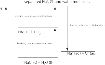
The solvation process can be considered as a three-step process:
- Breaking the solute-solute interactions
Examples
- Breaking the solvent-solvent interactions.
Examples
- Forming solvent-solute interactions – attraction between the solute and solvent particles.
Examples
The first two processes above are endothermic while the last process is exothermic. The overall thermodynamics is summarized in the following enthalpy level diagram; note that the overall enthalpy of solvation
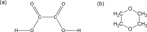
In this experiment, you will study the solubility of potassium dichromate ([latex]\textrm{K}_2\textrm{Cr}_2\textrm{O}_7[/latex]) or oxalic acid ([latex]\textrm{H}_2\textrm{C}_2\textrm{O}_4[/latex]) using two different solvents:
- pure water
- 70:30 water:1,4-dioxane (by volume) mixture
1,4-dioxane is (largely) nonpolar due to its symmetrical shape. The structures of both oxalic acid and 1,4-dioxane are illustrated below:
Effect of Temperature on Solubility
The temperature dependence of the solubility of substances are depicted graphically on a solubility curve.
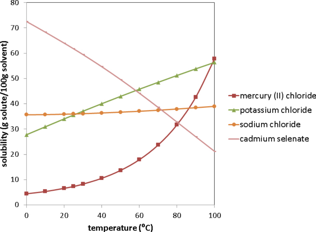
For many solid solutes in liquid solvents (as we see from everyday life) the solubility of the solute increases with temperature. However, this is not a hard and fast rule. For example, if you look at the solubility curve of cadmium selenate above, the solubility decreases as a function of temperature. As you could also see above, how much the solubility changes as a function of temperature varies significantly for different substances.
In this experiment, you will explore this for both of the solids that are studied in this experiment in both water and the water:1,4-dioxane mixture. Wwe will explore this in a more quantitative manner in the experiment Thermodynamics of the Solvation of Calcium Hydroxide.
Solubility Differences of a Solute in Different Solvents
As discussed above, the energetics of the solvation process involves a consideration of the solute-solute, solvent-solvent, and solute-solvent interactions. While entropic considerations mean that exothermic interactions overall are not necessary for solvation, it does mean that solvation is unlikely unless the solute-solvent interactions are comparable (or larger) than the solute-solute and solvent-solvent interactions.
Examples
Sodium chloride forms ion-dipole forces with water, which (mostly) counterbalances the ionic bonds (within sodium chloride) and hydrogen bonds (within water) that are broken. As a result, sodium chloride is soluble in water.
On the other hand, sodium chloride is insoluble in cyclohexane (C6H12), a non-polar solvent. This is because the energy required to break the ionic bonds in sodium chloride is much greater than the gain in van der Waals energy when sodium and chloride ions interact with cyclohexane molecules.
A common way of thinking about this is to use the like dissolves like approach (which largely holds though there are subtle nuances to be considered).
- Ionic/polar solutes are more likely to be soluble in polar solvents
- Non-polar solutes are more likely to be soluble in non-polar solvents.
In this experiment, you will compare the solubility of each of the two solutes in the two solvent systems studied, and evaluate the difference in the context of this discussion.
Procedures
In this experiment, you will be assigned to measure the solubility curves for either potassium dichromate or oxalic acid. You will then (before leaving the lab) share data with another group of students who did the measurements for the other solute.
- Volumes of solvent can be measured using a 5 mL graduated pipet.
- Part C must be completed in a fume hood.
- Students may be asked to complete the experiment in a different order from that listed here to help traffic control. This will not affect the results of the experiment.
- Throughout this experiment, it is important to stir the test tube continuously in a gentle manner such that the temperature throughout the test tube. On the other hand, you must do it in a manner such that you don’t break the test tube.
Part A: Solubility of a Solid Solute in Water
- On a piece of weighing paper, weigh out (as assigned) either 3.1-3.3 g oxalic acid or 2.8-2.9 g potassium dichromate. Be sure to record the exact mass of your solute.
- Add the solid into a medium sized test tube.
- Using a graduated pipet, add 5.0 mL deionized water into the test tube. Use a test tube holder to clamp the test tube.
- Place the test tube into a 400 mL beaker of warm tap water. Begin heating the beaker on a hot plate, using the beaker as a water bath.
- Stir the mixture in the test tube regularly using the thermometer, keeping the test tube in the water bath until all of the solid has dissolved. You may also wish to stir (using a glass rod) the beaker of hot water from time to time.
- When all of the solid has dissolved, take the test tube out of the hot water beaker. Continue stirring the test tube gently while the test tube cools.
- Record the temperature when you first see for certain crystals of solute come out of solution. Be careful not to confuse contaminants (e.g. specks of dust) with the solute.
- Add 3.0 mL deionized water into the test tube. Place the test tube back into the hot water beaker and repeat steps 5-7.
- Add 2.0 mL deionized water into the test tube. Place the test tube back into the hot water beaker and repeat steps 5-7.
- Add 3.0 mL deionized water into the test tube. Place the test tube back into the hot water beaker and repeat steps 5-7.
Part B: Solubility of Your Solute in a Dilute Solution
- Prepare a 400 mL beaker containing ice. You may wish to add some salt to the ice as well.
- Weigh out and place into a clean, dry test tube approximately 0.9 g of your assigned solid.
- Add 5.0 mL of deionized water into the test tube.
- Repeat steps 5-7 from Part A. If the solute is still completely dissolved at room temperature, place the test tube into the ice/salt bath and allow the mixture to cool until crystals of your solid are observed.
- Add 2.0 mL deionized water into the test tube and repeat step 14 twice.
Part C: Solubility of Your Solute in a Water:1,4-Dioxane Mixture
-
- At your lab bench, weigh out and place in a clean, dry test tube your assigned solid. As before, masses near the lower end of these ranges would be more appropriate.
- 1.4-1.6 g potassium dichromate
- 3.2-3.5 g oxalic acid
- Move your test tube, graduated pipet, two 400 mL beakers (one containing your ice bath), thermometer, and test tube holder to a space in the fume hood.
- Measure out 5.0 mL of the 70:30 (v/v) water:dioxane mixture into the test tube.
- Repeat step 14 from Part B above.
- Add 3 mL of the 70:30 (v/v) water:dioxane mixture to the test tube and repeal step 14 from Part B again.
- Repeat step 20 two more times.
- Be sure to obtain the experimental data on the solid you did not study from another pair of students before you leave the laboratory.
- At your lab bench, weigh out and place in a clean, dry test tube your assigned solid. As before, masses near the lower end of these ranges would be more appropriate.
Waste Management
All waste must be collected and discarded into appropriate beakers placed in the fume-hood. There will be two separate waste beakers: one for waste containing oxalic acid and one for waste cotnaining potassium dichromate.
Data Analysis
For this experiment, you will need to first determine the solubility of the solid for each trial. Since the volume of the solvent was measured at room temperature, the density value used should be that at room temperature (25°C):
| Solvent | Density (g/mL) |
| water | 0.9975 |
| 70:30 (v/v) water:dioxane mixture | 1.023 |
Using these density values, calculate the mass of solvent used for each data point in this experiment. Note that the volume of solvent used should be the total volume of solvent added, not the amount added at that point.
Examples
If you have first added 10.0 mL water, then added another 5.0 mL water, the total volume of solvent added is [latex]10.0 \textrm{ mL} + 5.0 \textrm{ mL}= 15.0\textrm{ mL}[/latex]. You will then calculate the mass of the solvent as:
[latex]?\textrm{ g} = 15.0\textrm{ mL} \times \frac{0.9975\textrm{ g}}{\textrm{mL}} = 14.96 \textrm{ g}[/latex]
From this, calculate the concentration of the solute (in g solute/(100 g solvent)) for each data point.
Examples
If the mass of solute is 5.912 g (should be the same for the entire part) and for that given trial you had 15.0 mL water (and hence the mass of solvent is 14.96 g from above), the concentration of this solution is
\begin{eqnarray}
? \frac{\textrm{g solute}}{100\textrm{ g solvent}} &=& 100\mbox{ g solvent} \times \frac{5.912\textrm{ g K}_2\textrm{Cr}_2\textrm{O}_7}{9.98\textrm{ g H}_2\textrm{O}} \\
&=& 59.3\textrm{ g solute/100 g solvent}
\end{eqnarray}
Graphs
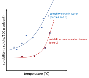
Make two plots (one for each solute) where you plot the solubility in each solvent (along the y-axis) as a function of temperature (along the x-axis).
On each graph, there should be two data sets along the same axes.
- The solute in water (Parts A and B). The data for both those parts (for a given solute) should fall along a single, smooth curve.
- The solute in a 70:30 water:1,4-dioxane mixture (Part C). The data for this part (for a given solute) should fall on a separate, smooth curve.
Each set should be plotted with different symbols, and a smooth curve to illustrate the trend in the data (as best as possible) should be included to guide the eye for each set as shown in the illustration below. It is common for there to be anomalous data points in this data, so you should not expect the curve to go through every data point or for every “jump” to follow the overall trend.
- Well, there are supersaturated solutions where there is a greater amount of solute dissolved than what is found in the solubility. However, such solutions are not thermodynamically stable and will not be considered in this experiment. ↵
