47 Gaussian-Seidel Iteration
Recall that in Part VI: Chapter 27, we discussed how to solve a system of linear equations by using Gaussian elimination. In this section, we will discuss the Gaussian-Seidel Iteration process which is another method we can use to solve systems of linear equations.
When working with only a few equations, Gaussian elimination is preferred between the two methods. But when working with many equations, the Gaussian-Seidel iteration method may actually be the better method [9].
With this method, it is necessary that we arrange the equations in the proper order [9]. Consider the following matrix representation of a system of linear equations.
![Rendered by QuickLaTeX.com \[\begin{bmatrix} a_{11}x_1 & a_{12}x_2 & \cdots & a_{1n}x_n & c_1 \\ a_{21}x_1 & a_{22}x_2 & \cdots & a_{2n}x_n & c_2 \\ \vdots & \vdots & & \vdots &\vdots \\ a_{n1}x_1 & a_{n2}x_2 & \cdots & a_{nn}x_n & c_n \\ \end{bmatrix}\]](https://iu.pressbooks.pub/app/uploads/quicklatex/quicklatex.com-7c65795524cb63f9f71d0869502868e1_l3.png)
Looking at all of the coefficents for ![]() (
(![]() ), we want to find the coefficient with the largest magnitude (farthest from zero). The equation that contains the coefficient of
), we want to find the coefficient with the largest magnitude (farthest from zero). The equation that contains the coefficient of ![]() that has the largest magnitude is then moved to row 1. Looking at all of the coefficents for
that has the largest magnitude is then moved to row 1. Looking at all of the coefficents for ![]() (
(![]() ), we want the coefficient with the largest magnitude. The equation that contains the coefficient of
), we want the coefficient with the largest magnitude. The equation that contains the coefficient of ![]() that has the largest magnitude is then moved to row 2. This process is continued for each independent variable.
that has the largest magnitude is then moved to row 2. This process is continued for each independent variable.
It is important to realize that this method will not work for every system of linear equations. Sometimes, each iteration will actually lead us farther away from the solution (diverge) rather than lead us closer (converge). This is why it is a good idea to perform the Diagonal Dominance test before beginning the iterations. Supposing that our matrix above has been properly ordered, consider the following inequalities.
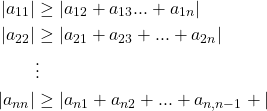
If at least ![]() of these inequalities are true and at least one of these inequalities can be strictly greater than and still true, then we are guaranteed that the Gaussian-Seidel iteration method will converge to the solution [9]. However, it is not the case that failing to pass this test guarantees divergence. It is possible to fail the test and still converge [9].
of these inequalities are true and at least one of these inequalities can be strictly greater than and still true, then we are guaranteed that the Gaussian-Seidel iteration method will converge to the solution [9]. However, it is not the case that failing to pass this test guarantees divergence. It is possible to fail the test and still converge [9].
After rearranging our equations, we must pick some initial values, one for each independent variable, to start the iterations. However, unlike the Newton-Raphson or Secant rule methods, our choices for the initial values will not make a difference in whether we get closer to the solution with each iteration or not [9].
After reordering equations, performing the Diagonal Dominance test, and choosing initial values, we are ready to begin our iterations. Consider this properly-ordered matrix.
![Rendered by QuickLaTeX.com \[\begin{bmatrix} a_{11}x_1 & a_{12}x_2 & \cdots & a_{1n}x_n & c_1 \\ a_{21}x_1 & a_{22}x_2 & \cdots & a_{2n}x_n & c_2 \\ \vdots & \vdots & & \vdots &\vdots \\ a_{n1}x_1 & a_{n2}x_2 & \cdots & a_{nn}x_n & c_n \\ \end{bmatrix}\]](https://iu.pressbooks.pub/app/uploads/quicklatex/quicklatex.com-7c65795524cb63f9f71d0869502868e1_l3.png)
The iteration for finding ![]() proceeds as follows.
proceeds as follows.
![]()
Basically, we solve the first of our ordered equations for ![]() and substitute in our values for every other variable. To find
and substitute in our values for every other variable. To find ![]() , we solve the second of our ordered equations for
, we solve the second of our ordered equations for ![]() and substitute in our values for every other variable. Once this is done for every variable, our first iteration is complete. We then do this process again for our second iteration and so on.
and substitute in our values for every other variable. Once this is done for every variable, our first iteration is complete. We then do this process again for our second iteration and so on.
Let’s work through an example to clarify this process along with the Diagonal Dominance test. This problem is one I completed for this paper and comes from Hiestand [9].
Consider the equation set

Show that this satisfies the convergence criteria for the Gaussian-Seidel method of solving equations. Rearrange the equations as needed. Then, assume starting values of ![]() . Then perform three iterations of Gaussian-Seidel.
. Then perform three iterations of Gaussian-Seidel.
Solution
We first need to rearrange our equations. The coefficients of ![]() are 4, 9, and 7. Because 9 is the furthest from 0, the equation containing
are 4, 9, and 7. Because 9 is the furthest from 0, the equation containing ![]() should be the first equation. Of the coefficients of
should be the first equation. Of the coefficients of ![]() , 8 is the furthest from 0 so the equation containing
, 8 is the furthest from 0 so the equation containing ![]() should be the second equation. Finally, of the coefficients of
should be the second equation. Finally, of the coefficients of ![]() , -10 is the furthest from 0 so the equation containing
, -10 is the furthest from 0 so the equation containing ![]() should be the third equation. Thus, our ordered system of equations is
should be the third equation. Thus, our ordered system of equations is

Now that we have reordered our equations, we are ready for the Diagonal Dominance test. We have that

Because we have at least two equations where the left side is greater than or equal to the right side and at least one equation where the left side is strictly greater than the right side, this system satisfies the convergence criteria for the Gaussian-Seidel method by the Diagonal Dominance test.
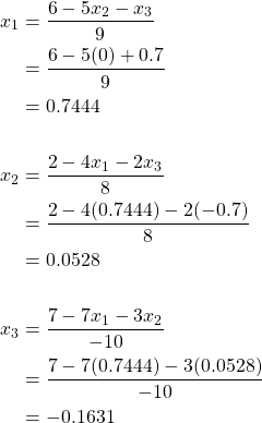
With starting values ![]() , our first iteration for
, our first iteration for ![]() is
is
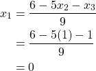
Because ![]() is now 0, our first iteration for
is now 0, our first iteration for ![]() is
is
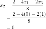
Because ![]() , our first iteration for
, our first iteration for ![]() is
is
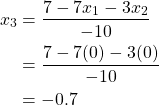
Let’s now plug these values into our original equations to see how accurate they are.

Starting our second iteration, we have ![]() ,
, ![]() , and
, and ![]() .
.
Plugging in these values to our original equations, we have

For our third iteration, we have ![]() ,
, ![]() , and
, and ![]() .
.
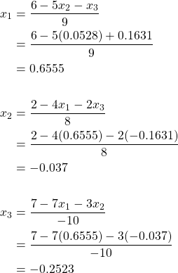
Plugging in these values to our original equations, we have

As we can see, each iteration brings us closer to the solution of this equation, and after three iterations we have

