Limits and Continuity

Abigail Huettig

21 Limits and Continuity

We already mentioned limits and continuity of functions in Part I: Chapter 1. Instead of reiterating what was already discussed, we will introduce some new ideas, going deeper into limits and continuity. When we discussed limits before, we never actually gave a formal definition. So, we will start by defining limits using the following definition given by Abbott [1].

Definition IV.20
Let $f:A\rightarrow\mathbb{R}$ , and let $c$ be a limit point [see limit point definition in chapter 19] of the domain $A$ . We say that $\lim_{x\to c}f(x)=L$ provided that, for all $\epsilon>0$ , there exists a $\delta>0$ such that whenever $0<|x-c|<\delta$ (and $x\in A$ ) it follows that $|f(x)-L|<\epsilon$ .

Let’s now go through an example of how to use this definition. This example is a homework problem that I completed for Introduction to Analysis [6].

Example 45
Show that $\displaystyle\lim_{x\to 7}(13x-42)=49$ .

Proof.
Let $\epsilon>0$ .

$\begin{align*} |f(x)-L|&=|13x-42-49|\\ &=|13x-91|\\ &=13|x-7| \end{align*}$

Let $\delta=\displaystyle\frac{\epsilon}{13}$ . So, $0<|x-7|<\delta$ implies

$\begin{align*} |f(x)-L|&=13|x-7|\\ &<13\delta\\ &=13\left(\frac{\epsilon}{13}\right)\\ &=\epsilon \end{align*}$

Therefore, $\displaystyle\lim_{x\to 7}(13x-42)=49$ .

When finding limits, we can combine our approaches from Calculus and Analysis. Calculus allows us to find a good candidate for the limit by doing what we did in Part I: Chapter 1. Analysis then allows us to prove that this candidate is in fact the limit by using definition IV.20 as just shown above. Now, we will explore continuity from an analysis perspective, looking at the Intermediate Value Theorem and uniform continuity.

Intermediate Value Theorem

We will start by presenting this theorem as it is given by Abbott [1].

Theorem IV.21 (Intermediate Value Theorem)

Let $f:[a,b]\rightarrow\mathbb{R}$ be continuous. If $L$ is a real number satisfying $f(a)<L<f(b)$ or $f(a)>L>f(b)$ , then there exists a point $c\in (a,b)$ where $f(c)=L$ .

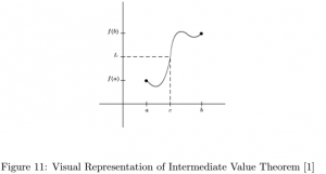
Let’s consider the image from Abbott above as we discuss what this theorem is saying. We have a continuous function $f(x)$ whose domain is the closed interval $[a,b]$ . So the graph of this function will have two endpoints, $(a,f(a))$ and $(b,f(b))$ . There is also a real number $L$ between $f(a)$ and $f(b)$ . Now picture a horizontal line at $L$ . Regardless of what continuous function we draw to connect the two endpoints, it will intersect the horizontal line at some point, and we can label this point as $(c,L)$ . Therefore, there exists a point $c$ in the interval $(a,b)$ where $f(c)=L$ .

Let’s now look at an example of how this theorem can be used. The following problem is from Abbott and is a proof I completed as homework for Introduction to Analysis [1].

Example 46
Show that it is impossible to have a continuous function defined on all of $\mathbb{R}$ with range equal to $\mathbb{Q}$ .

Proof.
Consider a continuous function $f(x)$ defined on all of $\mathbb{R}$ with a range equal to $Q$ . That is, $f:\mathbb{R}\rightarrow\mathbb{Q}$ is continuous. Because $f(x)$ is continuous on every point in $\mathbb{R}$ , $f(x)$ is continuous on every point in a closed interval $[a,b]\subset\mathbb{R}.$ So, $f:[a,b]\rightarrow\mathbb{Q}$ is continuous. By Corollary IV.4.1 in chapter 19, there exists $L\in\mathbb{I}$ where

$f(a)<L<f(b)$

or

$f(a)>L>f(b).$

By the Intermediate Value Theorem, there exists $c\in (a,b)$ such that

$f(c)=L.$

This contradicts the range being equal to $\mathbb{Q}$ since $L\notin\mathbb{Q}$ . Thus, $f:[a,b]\rightarrow\mathbb{Q}$ is not continuous which implies $f:\mathbb{R}\rightarrow\mathbb{Q}$ is not continuous. Therefore, it is impossible to have a continuous function defined on all of $\mathbb{R}$ with range equal to $\mathbb{Q}$ .

So, this is the Intermediate Value Theorem (IVT). It is an example of an idea that seems so clear and obvious that mathematicians used it for years without a formal proof of its being true [1]. There does exist a proof for it now, but we will not cover it here. Instead, let’s move on to uniform continuity.

Uniform Continuity

We already introduced a definition for continuity of a function in Part I: Chapter 1, but now we will look at another definition for continuity of a function provided by Abbott [1].

Definition IV.22
A function $f:A\rightarrow\mathbb{R}$ is continuous at a point $c\in A$ if, for all $\epsilon>0$ , there exists a $\delta>0$ such that whenever $|x-c|<\delta$ (and $x\in A$ ) it follows that $|f(x)-f(c)|<\epsilon$ .

From the Calculus perspective, we said that a function $f(x)$ was continuous at $c$ if

$\lim_{x\rightarrow c}f(x)=f(c)$

given that the limit exists and $f(c)$ is defined. So, if $f(x)$ is continuous at $c$ and the limit equals $L$ , then

$L=f(c).$

Then, we can substitute $f(c)$ for $L$ in definition IV.20, and we get the definition of continuity given above with a couple of differences.

First, we do not state that $c$ is a limit point in the continuity definition. This is because the limit at $c$ would not exist if $c$ were not a limit point. Since we are substituting $f(c)$ in for $L$ , it is given that the limit exists so it would be redundant to restate that $c$ must be a limit point.

Second, in the limit definition, it is stated that

$0<|x-c|<\delta$

whereas the continuity definition says that

$|x-c|<\delta.$

The difference is that the limit definition defines $x$ as not equal to $c$ . The reason is that the limit can still exist at $c$ even if the function is not defined at $c$ . So, if we let $x$ equal $c$ and $f(c)$ happens to be undefined,

$|f(x)-L|=|f(c)-L|<\epsilon$

would not make sense. However, if a function is continuous at $c$ , it follows that $f(c)$ is defined. So, we do not have to restrict $x$ to not being equal to $c$ .

Thus, using definition IV.20 along with the definition of continuity from Calculus, we arrive at the definition of continuity given above.

Uniform continuity is similar but a bit stricter than continuity. The definition of uniform continuity is given by Abbott as follows [1].

Definition IV.23
A function $f:A\rightarrow\mathbb{R}$ is uniformly continuous on $A$ if for every $\epsilon>0$ there exists a $\delta>0$ such that for all $x,y\in A$ , $|x-y|<\delta$ implies $|f(x)-f(y)|<\epsilon.$

The definitions of continuity and uniform continuity look very similar which makes it difficult to understand the difference between the two. As mentioned before, uniform continuity is a stricter form of continuity so a function can be continuous without being uniformly continuous. But if a function is uniformly continuous, it follows that the function is continuous.

A function is continuous if it is continuous at every point $c$ in its domain. So for a fixed $\epsilon>0$ , $\delta>0$ can take on different values depending on $c$ , and the function will still be continuous. The difference is that for a function to be uniformly continuous there must exist a single $\delta>0$ for a fixed $\epsilon>0$ for all $c$ in the domain [1].

We also have a theorem that helps with showing that a function is not uniformly continuous. What we use to disprove uniform continuity is the Sequential Criterion for Absence of Uniform Continuity. Abbott states it as follows [1].

Theorem IV.24 (Sequential Criterion for Absence of Uniform Continuity)

A function $f:A\rightarrow \mathbb{R}$ fails to be uniformly continuous on $A$ if and only if there exists a particular $\epsilon_0>0$ and two sequences $(x_n)$ and $(y_n)$ in $A$ satisfying

$|x_n-y_n|\rightarrow 0$

but

$|f(x_n)-f(y_n)|\geq \epsilon_0.$

If we can find two sequences, $(x_n)$ and $(y_n)$ , in the domain of a function $f(x)$ such that the sequence $|x_n-y_n|$ converges to 0 and the sequence $|f(x_n)-f(y_n)|$ is bounded below by a positive number, then $f(x)$ is not uniformly continuous.

Let’s now look at an example that demonstrates how to prove a function is not uniformly continuous. This is a homework problem I completed for Introduction to Analysis that comes from Abbott [1].

Example 47
Show that the continuous function $f(x)=x^4$ is not uniformly continuous.

Proof.
Let $f(x)=x^4$ with domain $\mathbb{R}$ . Let $\epsilon_0=6$ , $(x_n)=n$ and $(y_n)=n+\frac{1}{n}.$
If

$\begin{align*} a_n&=|x_n-y_n|\\ &=\left|n-n-\frac{1}{n}\right|\\ &=\left|-\frac{1}{n}\right|\\ &=\frac{1}{n} \end{align*}$

then $\lim (a_n)=0.$ Additionally,

$\begin{align*} |f(x_n)-f(y_n)|&=\left|n^4-n^4-4n^2-\frac{4}{n^2}-\frac{1}{n^4}-6\right|\\ &=4n^2+\frac{4}{n^2}+\frac{1}{n^4}+6\\ &>6\\ &=\epsilon_0 \end{align*}$

$\forall\, n\in \mathbb{N}$ . By Theorem IV.24, $f(x)=x^4$ is not uniformly continuous on $\mathbb{R}$ .

Next, we will look at an example of how to show that a function is uniformly continuous. This example is a homework problem I completed for Introduction to Analysis that comes from Abbott [1].

Example 48
Show that $f(x)=x^4$ is uniformly continuous on any bounded subset of $\mathbb{R}$ .

Proof.
Consider the bounded subset of $\mathbb{R}$ $[-M,M]$ , where $M>0$ .

$\begin{align*} |f(x)-f(y)|&=|x^4-y^4|\\ &=|x+y||x-y||x^2+y^2|\\ &\leq (|x|+|y|)(|x^2|+|y^2|)(|x-y|) &&\text{Triangle Inequality}\\ &\leq 2M(2M^2)|x-y|\\ &=4M^3|x-y|\\ \end{align*}$

Let $\epsilon>0$ and $\delta=\displaystyle\frac{\epsilon}{4M^3}$ . If $|x-y|<\delta=\displaystyle\frac{\epsilon}{4M^3}$ , then

$\begin{align*} |f(x)-f(y)|&\leq 4M^3|x-y|\\ &<4M^3\left(\frac{\epsilon}{4M^3}\right)\\ &=\epsilon \end{align*}$

for all $x,y\in [-M, M]$ . Therefore, $f(x)$ is uniformly continuous on any bounded subset of $\mathbb{R}$ .

21 Limits and Continuity

Intermediate Value Theorem

Uniform Continuity

License

Share This Book