Lagrangian Polynomials

Abigail Huettig

36 Lagrangian Polynomials

In the real world, it is constantly observed that one event causes another or that one event is correlated with another in some way. Many times, experiments can be done to further explore these relationships, such as how temperature affects an element of the periodic table. But other times experiments are impossible, such as when human lives are on the line. For example, determining how different health conditions make a person more or less susceptible to a specific bacterium or virus should not be studied by purposefully infecting people.

Mathematical models can give us information in areas where experiments cannot. By modeling, analyzing, and interpreting data mathematically, we can come up with explanations and make predictions without having to use experimentation. Then, the model can be tested and revised for accuracy when more data is given [8].

One way data is modeled is by finding a high-order polynomial that passes through each data point. In this section, we will focus on the Lagrangian form of the polynomial. Consider the following theorem from Giordano et al. [8].

Theorem VII.1 (Lagrangian Form of the Polynomial)

If $x_0,x_1,...,x_n$ are $(n+1)$ distinct points and $y_0,y_1,...,y_n$ are corresponding observations at these points, then there exists a unique polynomial $P(x)$ , of at most degree $n$ , with the property that

$y_k=P(x_k)\,\,\text{for each}\,\,k=0,1,...n.$

This polynomial is given by

$P(x)=y_0L_0(x)+...+y_nL_n(x)$

where

$L_k(x)=\frac{(x-x_0)(x-x_1)...(x-x_{k-1})(x-x_{k+1})...(x-x_n)}{(x_k-x_0)(x_k-x_1)...(x_k-x_{k-1})(x_k-x_{k+1})...(x_k-x_n)}.$

This theorem is pretty straightforward, but let’s do one example to see this theorem in action. This problem is one I completed for Mathematical Models/Applications 2 and comes from Giordano et al. [8].

Example 71
Consider the following data set:

Fit the data into the Lagrange Interpolation Polynomial.

Solution
To find the polynomial all we have to do is plug the data points into the formula given in Theorem VII.1. Because we have six data points, the following polynomial has a degree of 5.

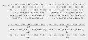
It is clear that this polynomial passes through each of the data points. For each $x_i$ , $L_j(x_i)$ is equal to zero when $i$ is not equal to $j$ . What is left is

$P(x_i)=L_i(x_i)y_i.$

Because $L_i(x_i)$ is equal to one, we are left with

$P(x_i)=y_i.$

The Lagrange Polynomial model is useful in that it allows us to predict the corresponding $y$ -value of a given $x$ -value. The drawback is that this $x$ must be between $x_0$ and $x_n$ . For example, in our problem above, we could predict the corresponding $y$ -value to $x$ equals 3 by finding $P(3)$ , and our prediction would be quite accurate. However, using this polynomial to try and predict the corresponding $y$ -value for $x$ equals -1 or $x$ equals 7 will likely lead to predictions that are not accurate.

Another problem with using the Lagrangian Polynomial is that as the number of data points increases so does the order of the polynomial. There are a couple of disadvantages with using a high-order polynomial as we will see. One way to remedy this is to use linear and cubic splines.

36 Lagrangian Polynomials

License

Share This Book