The Trapezoid Rule

Abigail Huettig

43 The Trapezoid Rule

Recall that in Part I: Chapter 3, we mentioned that the integral of a function could be thought of as the area between the horizontal axis and the graph of the function. We are now going to take a more detailed look at this idea.

Consider the following diagram.

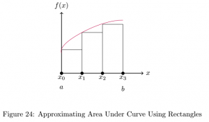
The integral that this figure represents is

$\int_a^b f(x)\, dx.$

What the integral does is partition the interval $[a, b]$ into smaller intervals

$[x_0, x_1], [x_1, x_2], [x_2, x_3]$

each with a length of $\Delta x$ . Then, $\Delta x$ is multiplied by the function evaluated at the beginning point of each interval, and the products are added together. That is,

$\begin{align*} \int_a^b f(x)\, dx &\approx \Delta x\cdot f(x_0)+\Delta x\cdot f(x_1)+\Delta x\cdot f(x_2)\\ &=(x_1-x_0)\cdot f(x_0)+(x_2-x_1)\cdot f(x_1)+(x_3-x_2)\cdot f(x_2) \end{align*}$

As we can see, this equation is the same one we would use if we were asked to find the areas of the rectangles and add them together. Thus, the integral is approximately the combined area of these rectangles. Unfortunately, the problem with using these rectangles is that they do not give a very good approximation of the area under the curve because there are large gaps between the rectangles and the curve.

This problem can be fixed by making $\Delta x$ very, very small which results in many, very thin rectangles. Because these rectangles are so thin, they provide a much better approximation of the area under the curve that differs only slightly from the exact area. Because finding the areas of each of these rectangles and adding them together is a difficult if not impossible task, we evaluate the integral using the Fundamental Theorem of Calculus, which is stated in chapter 3.

However, using this theorem requires that we find the antiderivative of the function, which can sometimes be extremely difficult. This is why the trapezoid rule is important. It enables us to bypass the antiderivative and gives us a better approximation of the area than the rectangle method can give.

Visually, the trapezoid rule uses trapezoids as opposed to rectangles. Consider the following diagram.

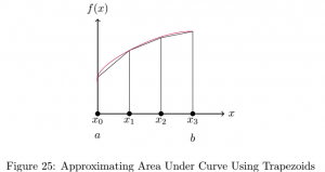
Recall that the area of a trapezoid is the average of the lengths of the parallel sides multiplied by the distance between the parallel sides. Using figure 25, the area of the trapezoid is

$\frac{f(x_i)+f(x_{i+1})}{2}\cdot \Delta x$

where $\Delta x$ is the distance between $x_i$ and $x_{i+1}$ .

The way we approximate an integral using the trapezoid rule is similar to how we did it with the rectangles. We partition the interval into smaller intervals of equal length, but instead of using rectangles, we use trapezoids. We then find the area of each trapezoid and add the areas together.

From figures 24 and 25, it is clear that the trapezoid rule provides a better approximation than the rectangle method because there is less space between the trapezoids and the curve than there is between the rectangles and the curve.

Let’s now work through an example I completed for this paper that comes from Hiebert [9].

Example 77
Consider the following integral:

$\int_0^{0.5} \sqrt{1-x^2}\, dx.$

Evaluate this integral with 4 intervals, using the trapezoid rule.

Solution
We want to break the interval $[0, 0.5]$ into 4 equally sized intervals. So, our intervals are

$[0, 0.125], [0.125, 0.25], [0.25, 0.375], [0.375, 0.5].$

Next, we use the formula

$\frac{f(x_i)+f(x_{i+1})}{2}\cdot \Delta x$

on each interval to find the area of each trapezoid and add the areas together. So, what we have is

$\begin{align*} \int_0^{0.5} \sqrt{1-x^2}\, dx&\approx \frac{f(0)+f(0.125)}{2}\cdot 0.125+\frac{f(0.125)+f(0.25)}{2}\cdot 0.125 \\ &+\frac{f(0.25)+f(0.375)}{2}\cdot 0.125+\frac{f(0.375)+f(0.5)}{2}\cdot 0.125\\ \text{}\\ &=0.0625\cdot (f(0)+f(0.125)+f(0.125)+f(0.25)\\ &+f(0.25)+f(0.375)+f(0.375)+f(0.5))\\ \text{}\\ &=0.0625\cdot (f(0)+2f(0.125)+2f(0.25)+2f(0.375)+f(0.5))\\ &\approx 0.0625\cdot (1+1.98431+1.93649+1.85405+0.86603)\\ \text{}\\ &=0.477555 \end{align*}$

Therefore,

$\int_0^{0.5} \sqrt{1-x^2}\, dx\approx 0.477555$

by the trapezoid rule.

Whenever we find an approximation, we want to find how close it is to the exact answer. In our next section, we will do just that by calculating the Trapezoid Rule errors.

Trapezoid Rule Errors

Since the trapezoid rule approximates the integral, it is helpful to know how much of a difference there is between the approximated area and the exact area. The formula for the error, known as truncated error, is given by Hiestand as follows [9].

(1) $\begin{align*} E_{\text{TRUN}}=-\frac{(\Delta x)^2\cdot (b-a)\cdot f''(x)}{12} \end{align*}$

Using this formula, we can calculate two different errors, the maximum error and the average error.

The Maximum Error
The first method is the maximum error method, which gives us the largest possible error. That is, the true error between the exact and approximated value will be less than or equal to the maximum error. To find this error, we first choose $c$ in the interval $[a,b]$ such that the absolute value of $f''(c)$ is greater than or equal to the absolute value of $f''(x)$ for all $x$ in $[a,b]$ [9]. Then, we substitute $f''(c)$ for $f''(x)$ in equation 1 above. This gives us

(2) $\begin{align*} E_{\text{TRUN, max}}=-\frac{(\Delta x)^2\cdot (b-a)\cdot f''(c)}{12}, \end{align*}$

which is the formula for the maximum error [9].

In the following example, we are going to approximate the maximum error for our approximation from example 77.

Example 78
Consider the following integral:

$\int_0^{0.5} \sqrt{1-x^2}\, dx.$

Estimate the maximum error when $\Delta x=0.125$ .

Solution
We have that

$\begin{align*} f(x)&=\sqrt{1-x^2}\\ \text{}\\ f'(x)&=\frac{d}{dx}(1-x^2)^{\frac{1}{2}}\\ &=\frac{1}{2}(1-x^2)^{-\frac{1}{2}}(-2x) &&\text{Chain Rule}\\ &=\frac{-x}{\sqrt{1-x^2}}\\ \text{}\\ f''(x)&=\frac{d}{dx}\left(\frac{-x}{\sqrt{1-x^2}}\right)\\ &=\frac{\sqrt{1-x^2}\frac{d}{dx}(-x)-(-x)\frac{d}{dx}\sqrt{1-x^2}}{(\sqrt{1-x^2})^2} &&\text{Quotient Rule}\\ &=\frac{-\sqrt{1-x^2}-\frac{x^2}{\sqrt{1-x^2}}}{(\sqrt{1-x^2})^2}\\ &=\frac{-1-\frac{x^2}{1-x^2}}{\sqrt{1-x^2}}\\ &=-\frac{1}{\sqrt{1-x^2}}-\frac{x^2}{(1-x^2)^{\frac{3}{2}}} \end{align*}$

Below is the graph of $f''(x)$ restricted to the domain $[0, 0.5]$ .

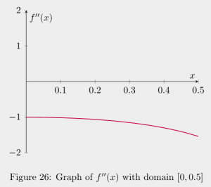
The $x$ -value for which the absolute value of $f''(x)$ is greatest is 0.5 since the point $(0.5, f''(0.5))$ is the farthest from the $x$ -axis. So, we should let $c=0.5$ . Plugging everything into equation 2 above, we have

$\begin{align*} E_{\text{TRUN, max}}&=-\frac{(\Delta x)^2\cdot (b-a)\cdot f''(c)}{12}\\ &=-\frac{(0.125)^2\cdot (0.5-0)\cdot f''(0.5)}{12}\\ &\approx -\frac{(0.125)^2\cdot 0.5\cdot (-1.5396)}{12}\\ &\approx 0.001002 \end{align*}$

Therefore, $E_{\text{TRUN, max}}\approx 0.001002.$

Average Error
The other error we can calculate is the average error. According to Hiebert, the formula

$f^N(x)=\frac{f^{N-1}(b)-f^{N-1}(a)}{b-a}$

gives us the average of the $N$ th derivative of a function over the interval $[a,b]$ [9]. So,

$f''(x)=\frac{f'(b)-f'(a)}{b-a}.$

To get the formula for the average error, we substitute this equation into our formula for $E_{\text{TRUN}}$ (equation 1) [9].

(3) $\begin{equation*} \begin{split} E_{\text{TRUN, avg}}&=-\frac{(\Delta x)^2\cdot (b-a)\cdot \frac{f'(b)-f'(a)}{b-a}}{12}\\ &=-\frac{(\Delta x)^2\cdot (f'(b)-f'(a))}{12} \end{split} \end{equation*}$

In the following example, we are going to approximate the average error for our approximation from example 77.

Example 79
Consider the following integral:

$\int_0^{0.5} \sqrt{1-x^2}\, dx.$

Estimate the average error when $\Delta x=0.125$ .

Solution
We have that

$f'(x)=-\frac{x}{\sqrt{1-x^2}}.$

It follows that

$\begin{align*} f'(0)&=-\frac{0}{\sqrt{1-0^2}}\\ &=0 \end{align*}$

and

$\begin{align*} f'(0.5)&=-\frac{0.5}{\sqrt{1-0.5^2}}\\ &\approx -0.57735 \end{align*}$

Substituting everything into equation 3 above, we have

$\begin{align*} E_{\text{TRUN, avg}}&=-\frac{(\Delta x)^2\cdot (f'(b)-f'(a))}{12}\\ &=-\frac{(0.125)^2\cdot (f'(0.5)-f'(0))}{12}\\ &\approx -\frac{(0.125)^2\cdot (-0.57735-0)}{12}\\ &\approx 0.000752 \end{align*}$

Therefore, $E_{\text{TRUN, avg}}\approx 0.000752.$

The Trapezoid Rule developed from the need to have a more accurate approximation of an integral than the rectangle method could give. Similarly, Simpson’s Rules provide us with even better approximations than the Trapezoid Rule can give. We will look at both Simpson’s $\frac{1}{3}$ rule and $\frac{3}{8}$ rule, and which rule we use to approximate an integral depends on how many intervals we have.

43 The Trapezoid Rule

Trapezoid Rule Errors

License

Share This Book