Linear Programming

Abigail Huettig

35 Linear Programming

Linear programming focuses on optimization and minimization which is necessary in life, especially in business environments. Often, a company wants to know how to optimize profit or minimize cost or time. For example, a construction company may have a few different projects it could undertake but can only accomplish one. They want to know which option has the best combination of bringing in a lot of money while requiring as little expense to themselves as possible to optimize profit. Perhaps a manufacturing company has different options available for how to manufacture a product, and they want to know which way will work best for reducing cost and time of production while preserving the quality of the product. These are just a couple of many, many possible situations in which linear programming is needed. Any type of job or business may require information at one time or another that only linear programming can give.

It is important to realize that linear programming is not the only programming method in existence. There are others such as dynamic, integer, and nonlinear [10]. This is necessary because linear programming is not capable of solving every complex scenario that may arise. However, it is capable of solving a good number of them. This is why linear programming itself is quite complex and includes many different techniques, methods, and algorithms [10]. We will only be taking an introductory look at this type of programming, and the examples we see will be dealing with simpler problems that only deal with two or three linear equations. Keep in mind that these next few pages provide just a small glimpse into the power of linear programming and do not do justice to what it can do.

Finding Optimal Solutions by Graphing

We refer to solutions of both optimization and minimization problems as optimal solutions. These can be found a variety of ways, including graphing. The largest drawback of graphing is that it can be used only for problems with two or possibly three variables, making it an unusable method for most real-world problems. The benefit of the graphing method is that it gives a good introduction to linear modeling and presents a geometric view of how this type of modeling works. We will demonstrate the graphing method as well as introduce some common terminology of linear modeling in general by working through the following example. This is a problem I completed for Mathematical Models and Applications [5].

Example 69
The Apex Television Company has to decide on the number of 60- and 42-inch sets to be produced at one of its factories. Market research indicates that at most 30 of the 60-inch sets and 20 of the 42-inch sets can be sold per month. The maximum number of work hours available is 600 per month. A 60-inch set requires 20 work-hours and a 42-inch set requires 10 work-hours. Each 60-inch set sold produces a profit of $100 and each 42-inch set produces a profit of $80. A wholesaler has agreed to purchase all the television sets produced if the numbers do not exceed the maxima indicated by the market research.Formulate a linear programming model for this problem and use the graphical method to solve this model.

Solution

First, let’s create a table to organize the information that we have been given.

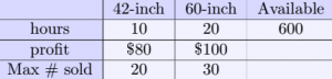
We need to make two decisions. The first is how many 42-inch sets to produce. The second is how many 60-inch sets to produce. So, let’s define our variables as

$x_1=\text{number of 42-inch produced}\text{ and } x_2=\text{number of 60-inch produced}.$

Because there are only 600 work hours available, we have the inequality

$10x_1+20x_2\leq 600.$

Additionally, because of the limit on how many sets of each type can be sold per month, we have

$0\leq x_1\leq 20\text{ and } 0\leq x_2\leq 30.$

Next, we graph all three inequalities with $x_1$ on the horizontal axis and $x_2$ on the vertical axis. (This graph was created using Desmos).

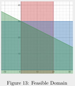
The only possible solutions for $x_1$ and $x_2$ that satisfy all of the inequalities are in the region where all three inequalities intersect (the dark region in the center). According to Hillier et al., if there exists at least one optimal solution, one of the corner points of this region will be an optimal solution. So, (0,0), (0,30), (20,20), or (20,0) is an optimal solution. If we let $Z$ be the total profit, we have the equation

$Z=80x_1+100x_2.$

All that is left to do is find $Z$ for each corner point and pick the point that yields the largest value of $Z$ .

$\begin{align*} &80(0)+100(0)=0\\ &80(0)+100(30)=3000\\ &80(20)+100(20)=3600\\ &80(20)+100(0)=1600 \end{align*}$

Therefore, the Apex Television Company should produce 20 of each type of TV set for a maximum profit of $3600.

Terminology
Let’s now go over some of the terminology that is commonly used for this type of problem. The variables are referred to as decision variables [10]. The equation that is to be maximized or minimized is the objective function ( $Z=80x_1+100x_2$ in our example) [10].The inequalities in the above problem are constraints. They are not always less than or equal to. It is possible to have greater than or equal to or just equal to [10]. Any solutions that satisfy all of the constraints are feasible solutions, and all that do not are infeasible solutions. The set that consists of all feasible solutions is the feasible region (the dark shaded region in our example). The corner points of the feasible region are known as corner-point feasible (CPF) solutions [10].

Number of Solutions
There may not always be an optimal solution. One possibility is that one constraint does not intersect all of the other constraints at some point, so there is no feasible solution because it is not possible to find a solution that satisfies all constraints. Another possibility is if the feasible region continues on indefinitely in some direction [10]. Suppose the only constraint we had for our example above was $0\leq x_1\leq 20$ . Because there are no constraints on $x_2$ , we can increase $x_2$ as much as we want which leads to $Z$ increasing without bound. There is no optimal solution because for every solution we can find a better one. It is also possible to have an infinite number of optimal solutions [10]. That is, for a maximum or minimum value of $Z$ , there may be an infinite number of choices for the decision variables that will yield $Z$ .

Corner Point Solutions
One thing that may not be clear is why an optimal solution, if such a solution exists, occurs at a corner point. Let’s look at our graph from the previous problem again. But this time, we will include the objective function with different values for $Z$ .

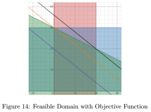
The following table provides information on what is shown in the graph.

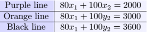
As you can see, as $Z$ increases, the graph of the objective function approaches the edge of the feasible region. We cannot increase $Z$ past 3600 because if we did, the objective function would no longer intersect the feasible region.

Regardless of what linear programming model we are solving with the graphing method, as $Z$ increases (or decreases), the objective function will approach a specific corner or side of the feasible region. The optimal solution will be where we can no longer increase (or decrease) $Z$ without it being infeasible. So, when $Z$ equals the maximum (or minimum) value, the objective function will intersect the feasible region at the very tip. If we have a single unique solution, they will intersect at a corner point. If there are infinite solutions, the objective function will intersect with an entire edge of the feasible domain, which is a line segment connecting two corner points. In either case, there exists at least one corner point that is an optimal solution.

Now that we have looked at the graphing method, we are going to move on to the Simplex method which enables us to find optimal solutions to objective functions involving many variables.

Tabular Simplex Method

The graphing method is great when we only have two decision variables. But many real-life situations will include many, many more. This is why we need other linear programming methods, such as the simplex method. The simplex method itself has many variations depending on the type and complexity of the problem needing to be solved. In this section, we will take an introductory look at the tabular simplex method, which can also function in different ways depending on the problem. Let’s work through an example to demonstrate the general process of this method. This is a homework problem I completed for Mathematical Models and Applications [5].

Example 70
Work through the simplex method in tabular form step by step to solve the following problem.Maximize $Z=2x_1-x_2+x_3$ , subject to

$3x_1+x_2+x_3\leq 6$

$x_1-x_2+2x_3\leq 1$

$x_1+x_2-x_3\leq 2$

and $x_1, x_2, x_3 \geq 0$ .

Solution
To make this problem easier to solve, we want to change the constraints from inequalities to equalities by introducing slack variables $x_4$ , $x_5$ , and $x_6$ [10]. We want our slack variables to equal the difference between the right and left sides of each inequality. That is, we will let

$\begin{align*} x_4 &= 6-3x_1-x_2-x_3\\ x_5 &=1-x_1+x_2-2x_3\\ x_6 &=2-x_1-x_2+x_3 \end{align*}$

which gives us the following three equations:

$\begin{align*} 3x_1+x_2+x_3+x_4 &= 6\\ x_1-x_2+2x_3+x_5 &=1\\ x_1+x_2-x_3+x_6 &=2 \end{align*}$

We also want to set the objective function equal to 0 by moving all of the terms on the right side to the left side which gives us

$Z-2x_1+x_2-x_3=0.$

Now we are ready to organize our information into a table known as the simplex tableau [10].

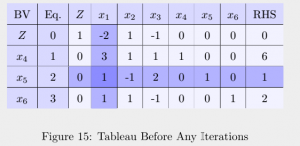
The first column contains the basic variables. The second column labels each equation with a number. Equation 0 is the objective function that was set equal to 0. Equation 1 is the first equality constraint, equation 2 the second, and equation 3 the third.The far right column is the right hand side of equations 0-3. Every other column gives the coefficients for each variable in each equation. For example, the coefficient of $x_3$ in equation 2 is 2.

Let’s take a moment to discuss basic variables in a little more detail. In the first tableau, the basic variables are always the slack variables along with the variable to be maximized or minimized. With every iteration of the process, one of the basic variables is replaced by a nonbasic variable. The variable being replaced is the leaving basic variable, and the one that becomes a basic variable is the entering basic variable [10].

There are four steps to every iteration.

Determine the entering basic variable.
Determine the leaving basic variable.
Change the value in the cell at the intersection of the entering basic variable column and leaving basic variable row to 1.
Change the values in every other cell of the entering basic variable column to 0.

So, our first step is to determine the entering basic variable. The entering basic variable is the one in equation 0 with the negative coefficient that has the largest absolute value [10]. Looking at figure 15 above, we see that -2 is the negative coefficient with the largest absolute value. So for our first iteration, the entering basic variable is $x_1$ .

Our next step is to determine the leaving basic variable, which we find using the minimum ratio test [10]. We take each positive coefficient in the column of the entering basic variable and divide it into the RHS number of the same row. The basic variable on the same row as the smallest quotient is the leaving basic variable. Looking at figure 15 above, we have the following equations.

$\begin{align*} 6\div 3 &= 2\\ 1\div 1 &= 1\\ 2\div 1 &= 2 \end{align*}$

Because 1 is the smallest quotient, $x_5$ is the leaving basic variable.

The third step is to change the value in the cell at the intersection of the entering basic variable column and leaving basic variable row to 1. We do this by multiplying the equation on the row of the leaving basic variable (referred to as the pivot row) by the multiplicative inverse of the number that is in that intersection cell. Recall from Part VI: Chapter 27 that multiplying by a nonzero constant in this way is an elementary row operation. Every time we need to change the value in a cell, we do so by elementary row operations. Looking at figure 15 above, we see that we do not have to multiply equation 2 by any constant because the value in the intersection cell is already 1.

The final step is to change the values in every other cell of the entering basic variable column to 0. Again, we do this with elementary row operations. Specifically, for each equation that does not have a 0 in the entering basic variable column, we will multiply the pivot row (equation 2 in this case) by a constant and add it to the equation. Looking at figure 15, we see that we have to

Multiply equation 2 by 2 and add it to equation 0.
Multiply equation 2 by -3 and add it to equation 1.
Multiply equation 2 by -1 and add it to equation 3.

After performing our first iteration, we have the following simplex tableau:

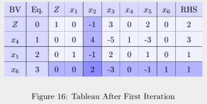
Notice that in the basic variables column $x_5$ was replaced by $x_1$ . Notice also that the column of coefficients for $x_1$ are now all zeros except for the row $x_1$ is now on.

Now, we perform the optimality test to determine whether we need another iteration. If every coefficient in equation 0 is nonnegative, then we have found the optimal solution. However, if there is at least one negative coefficient in equation 0, we must proceed with another iteration. Since $x_2$ has a negative coefficient, we must do another iteration.

Looking at figure 16 above, the entering basic variable is $x_2$ because the coefficient of $x_2$ in equation 0 is the only negative coefficient. Looking at the same tableau, we see that the leaving basic variable is $x_6$ because

$\begin{align*} 3\div 4&=\frac{3}{4}\\ 1\div 2 &=\frac{1}{2} \end{align*}$

The number in the cell that is at the intersection of the column of the entering basic variable and row of the leaving basic variable is 2 so we need to multiply equation 3 by $\frac{1}{2}.$ This results in the following tableau:

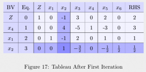
Now, we need to have a value of 0 in every other cell in the entering basic variable column. To do this, we need to

Add equation 3 to equations 0 and 2.
Multiply equation 3 by -4 and add it to equation 1.

After performing the second iteration, we have the following tableau:

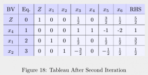
Because equation 0 has only nonnegative coefficients, we are done. Using the BV and RHS columns, we have an optimal solution of

$x_1=\frac{3}{2};\,\, x_2=\frac{1}{2};\,\, x_3=0; \,\,Z=\frac{5}{2}.$

Notice that $x_3$ is automatically 0 because it is not a basic variable.

The reason why we took so much time to work through this example is because the simplex method is so useful when solving maximization and minimization problems. We have only gone through one example, but we could go through so many more exploring how the simplex method is modified or used alongside other methods to solve complex problems. Another advantage of this method is that a computer system can be programmed to use it, which is extremely helpful when dealing with hundreds of decision variables.

One such program is Excel Solver. In the video below, I demonstrate how to use Excel Solver to solve linear programming problems.

Unfortunately, this is the end of our discussion of linear programming. We are now going to move on to a different area of modeling. We are going to see how we can find accurate models for modeling data, starting with Lagrangian Polynomials.

35 Linear Programming

Finding Optimal Solutions by Graphing

Tabular Simplex Method

License

Share This Book