
3 Integrals
The integral of a function  is usually thought of as the area between the graph of and the
  -axis. Although this is not a false idea, this description is only a piece of a much larger puzzle. It fails to unlock the true potential of integrals and prohibits a deeper understanding of what integrals are.
Integrals are, in essence, multiplication [5].
When we multiply, we are using repeated addition with numbers that remain fixed. For example,  is adding 30 fours together (
 ). But what happens if the four is changing? What if we had this:
![\[4+4^2+4^3+...+4^{30}?\]](https://iu.pressbooks.pub/app/uploads/quicklatex/quicklatex.com-56a77fef31e81a7b52c292414ddaed85_l3.png "Rendered by QuickLaTeX.com")
Here is where integration comes in.
Azad uses the example of  [5]. In real life, the speed will mostly likely be changing and will be different at different points in time. So, the equation would look like this:
![\[\text{distance}=\int s(t)\,\,dt ,\]](https://iu.pressbooks.pub/app/uploads/quicklatex/quicklatex.com-01c7f0877cd0673efb8437465decf210_l3.png "Rendered by QuickLaTeX.com")
where  is the speed at time
  . First, the integral breaks the total time into many tiny intervals. Then, the speed at time , where is the beginning of the interval, is multiplied by the length of the interval,
  , resulting in a tiny distance. This is done for each interval which results in a collection of tiny distances. Finally, the distances are added together to get the total distance [5]. All of this is done with this single equation:
![\[\text{distance}=\int s(t)\,\,dt.\]](https://iu.pressbooks.pub/app/uploads/quicklatex/quicklatex.com-13c8ba91558190a9634b30f175754926_l3.png "Rendered by QuickLaTeX.com")
Now let’s look at the formal definition provided by Larson and Edwards [15].
A function
 is an antiderivative of
  on an interval
  when
when  for all in .
In other words,
![\[\int f(x) \, dx=F(x).\]](https://iu.pressbooks.pub/app/uploads/quicklatex/quicklatex.com-b8f9baa2057e1545bcac232afaf384f0_l3.png "Rendered by QuickLaTeX.com")
It is important to understand that the definition says is an antiderivative of [15]. A function can have many antiderivatives. The reasoning behind this goes back to the constant rule where
![\[\frac{d}{dx}[c]=0\]](https://iu.pressbooks.pub/app/uploads/quicklatex/quicklatex.com-fdea638a495d2ebbb1cc04dcedc26f51_l3.png "Rendered by QuickLaTeX.com")
for some real number  . Consider
  . Some antiderivatives include
![\[F(x)=x^2, F(x)=x^2+5,\,\,\text{and}\,\, F(x)=x^2-5,764.\]](https://iu.pressbooks.pub/app/uploads/quicklatex/quicklatex.com-45377d53625ff4c2c5ebaee73d0cccef_l3.png "Rendered by QuickLaTeX.com")
When we take the derivative of any of these, we end up with because the constant always becomes 0. For this reason, we say the antiderivative of is
![\[F(x)=x^2+ C\]](https://iu.pressbooks.pub/app/uploads/quicklatex/quicklatex.com-16c7334ce9e7702a07853599d8093170_l3.png "Rendered by QuickLaTeX.com")
where  is a real number constant.
Just as we had derivative rules, we also have integral rules. A few of the basic ones are listed by Larson and Edwards as follows [15].


 , where
  is a constant

![\displaystyle\int [f(x)\pm g(x)]\, dx = \displaystyle\int f(x)\, dx \pm \displaystyle\int g(x)\, dx](https://iu.pressbooks.pub/app/uploads/quicklatex/quicklatex.com-e19060d65f24cd756717bae5aa5fd304_l3.png "Rendered by QuickLaTeX.com")
Let’s now work through an example to demonstrate some of these rules. This problem is one I completed for Calculus I and comes from Larson and Edwards [15].
Find the antiderivative of
 .
.
Solution

Therefore, the antiderivative of is
![\[F(x)=x+\frac{3}{x}-\frac{5}{3x^3}+C,\]](https://iu.pressbooks.pub/app/uploads/quicklatex/quicklatex.com-dd8af634b5183426edf89c6bdf8d04a3_l3.png "Rendered by QuickLaTeX.com")
where is a real number constant. That is, the derivative of
![\[F(x)=x+\frac{3}{x}-\frac{5}{3x^3}+C\]](https://iu.pressbooks.pub/app/uploads/quicklatex/quicklatex.com-ad5f000fca48a53bda78d7a5a6f1be5c_l3.png "Rendered by QuickLaTeX.com")
is .
An integral can come in many different forms, and often, we need to rewrite the integral so that it is in a form that can be integrated. One such strategy of rewriting integrals is integration by parts.
Integration by Parts
We have discussed how to integrate integrals using only the basic integration rules. But what happens when we have a function that cannot be integrated this way? Consider the function
![\[f(x)=x\sqrt{x-5}.\]](https://iu.pressbooks.pub/app/uploads/quicklatex/quicklatex.com-c72f3b1b53d033a6c73e3929b978dc7f_l3.png "Rendered by QuickLaTeX.com")
We can write as the product of two functions,
![\[u(x)=x\,\,\text{and}\,\,v(x)=\sqrt{x-5}.\]](https://iu.pressbooks.pub/app/uploads/quicklatex/quicklatex.com-d7feadb57e094c1bc544181961804c41_l3.png "Rendered by QuickLaTeX.com")
None of our basic integration rules tell us how to integrate products of functions so we need another method. This is where integration by parts comes in. Larson and Edwards give us the following theorem [15].
Theorem I.8
 and
and  are functions of and have continuous derivatives, then
![\[\int u\,dv=uv-\int v\,du.\]](https://iu.pressbooks.pub/app/uploads/quicklatex/quicklatex.com-ef23b8889938663eeea6be4430ff00da_l3.png "Rendered by QuickLaTeX.com")
Proof.
Let and be functions of with continuous derivatives.
![\begin{align*} \frac{d}{dx}[uv]&=u\frac{dv}{dx}+v\frac{du}{dx} &&\text{Product Rule}\\ \int\frac{d}{dx}[uv]\,dx&=\int u\frac{dv}{dx}\,dx+\int v\frac{du}{dx}\,dx &&\text{Integration Rule 5}\\ uv&=\int u\,dv+\int v\,du &&\text{dx's cancel}\\ \int u\,dv&=uv-\int v\,du &&\text{Rewrite}\\ \end{align*}](https://iu.pressbooks.pub/app/uploads/quicklatex/quicklatex.com-1a71298a905d8ba46276755f23ffc916_l3.png "Rendered by QuickLaTeX.com")
The process is to break the function we are trying to integrate into two separate parts, and  . Then, differentiate to get
  and integrate to get . Finally, subtract the integral of
  from the product
  .
.
Let’s now revisit our function
![\[f(x)=x\sqrt{x-5}\]](https://iu.pressbooks.pub/app/uploads/quicklatex/quicklatex.com-be6ad226008ecd6cd54ad55a08a908b6_l3.png "Rendered by QuickLaTeX.com")
and integrate it. This is a problem I completed for Calculus II that comes from Larson and Edwards [15].
Integrate

Solution
Let  and
and  It follows then that


So,

Therefore, the antiderivative of  is
is
![\[F(x)=\frac{2x(x-5)^{\frac{3}{2}}}{3}-\frac{4(x-5)^{\frac{5}{2}}}{15}+C.\]](https://iu.pressbooks.pub/app/uploads/quicklatex/quicklatex.com-2f02716f92a484f1fbeb467675b667e4_l3.png "Rendered by QuickLaTeX.com")
Keep in mind that there are many different methods and formulas for integration so integration by parts is not guaranteed to be the best method every time. But when faced with an integral that involves multiplying or dividing functions, it is a good method to try.
Another method that we have for rewriting integrals is trigonometric substitution.
Trigonometric Substitution
Trigonometric substitution is a very helpful method when integrating radicals. However, it is limited in that it only works with three general forms. The following summary of the forms and substitutions is from Larson and Edwards [15].
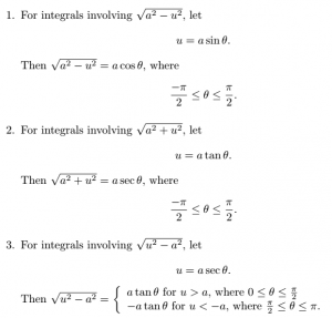
In order to understand why these substitutions work, we need a couple of Pythagorean identities [15]:


All that we need to do is substitute in and simplify using these Pythagorean identities. For example, the second form of trigonometric substitution looks like this:

The other two follow a similar line of reasoning. Now, we will go through a problem I completed for Calculus II from Larson and Edwards [15].
Find 
Solution
Let and  . By trigonometric substitution,

Additionally,

Substituting everything in, we have

Therefore, the antiderivative of  is
is
![\[F(x)=\sin^{-1}\left(\frac{x}{4}\right)+C.\]](https://iu.pressbooks.pub/app/uploads/quicklatex/quicklatex.com-48636258377487294afa89269a91c4ad_l3.png "Rendered by QuickLaTeX.com")
What we have been discussing so far is the indefinite integral. But there is another type of integral known as the definite integral.
Definite Integrals
The definite integral is denoted as
![\[\int_a^b\]](https://iu.pressbooks.pub/app/uploads/quicklatex/quicklatex.com-4e22a69a7e968835fac430ee8e268a91_l3.png "Rendered by QuickLaTeX.com")
This simply means that we are integrating over a closed interval ![[a,b]](https://iu.pressbooks.pub/app/uploads/quicklatex/quicklatex.com-fcda5ef4ae327e1afef79dc73df91703_l3.png "Rendered by QuickLaTeX.com") . We can evaluate such integrals using the following theorem given by Larson and Edwards [15].
. We can evaluate such integrals using the following theorem given by Larson and Edwards [15].
Theorem I.9 (The Fundamental Theorem of Calculus)
is continuous on the closed interval and is an antiderivative of on the interval , then
![\[\int_a^b f(x) \,dx=F(b)-F(a).\]](https://iu.pressbooks.pub/app/uploads/quicklatex/quicklatex.com-fcc4faa11945d5980a4524a793f1c097_l3.png "Rendered by QuickLaTeX.com")
We are now going to look at some of the many real-world applications of derivatives and integrals. Additionally, we will work through a real-world problem involving derivatives and another involving integrals, which demonstrates the Fundamental Theorem of Calculus.